The new Global Flood Monitoring (GFM) product of the Copernicus Emergency Management Service provides a continuous monitoring of floods worldwide by processing and analysing in near real-time all incoming Sentinel-1 Synthetic Aperture Radar (SAR) images acquired in Interferometric Wide Swath (IW) mode, and generating the eleven output layers of flood information that are listed in Table 1. The remainder of this Section presents the key technical details underlying the generation of the eleven GFM product output layers.
¶ Output layer “S-1 observed flood extent”
The GFM product output layer “S-1 observed flood extent” shows the flooded areas which are mapped in near real-time from Sentinel-1 (S-1) satellite imagery, as the difference between the GFM output layers “S-1 observed water extent” and “S-1 reference water mask”. The four flood mapping algorithms which are used by the GFM product to generate the output layer “S-1 observed flood extent” are described below.
¶ Flood mapping algorithm 1 (LIST)
GFM flood mapping algorithm 1 requires three main inputs: the most recent SAR scene to be processed, a previously recorded overlapping SAR scene acquired from the same orbit called reference SAR scene hereafter together with the corresponding “previous” ensemble flood extent map. As it is a change detection algorithm, it aims at detecting and mapping all increases and decreases of floodwater extent with respect to a reference one. A change detection approach is adopted because it allows to differentiate floodwater from permanent water bodies and, at the same time, filter out classes having water-like backscattering values such as shadows or smooth surfaces. Moreover, in order to reduce false alarms caused by different types of unrelated changes (e.g. vegetation growth), a reference image acquired close in time is used. Sentinel-1 fulfils well this latter requirement since it has a repeat cycle of 6 days. Moreover, to reduce false alarms and to speed-up the analysis, it uses as optional input data the exclusion mask and the HAND map. Each time a new Sentinel-1 scene is ingested and pre-processed, It0S1I_{t0}^{S1}It0S1, the algorithm processes the pair of S1 scenes consisting of the new image, It0S1I_{t0}^{S1}It0S1, and the previously recorded overlapping Sentinel-1 image acquired from the same orbit, It0−1S1I_{t0-1}^{S1}It0−1S1, and it provides the new floodwater map, FMt0FM_{t0}FMt0, updating the previous floodwater map, FMt0−1FM_{t0-1}FMt0−1. In the end, the algorithm makes use of the changes it mapped to update the most recently computed ensemble flood extent map (FMt0−1FM_{t0-1}FMt0−1).
Since the preprocessed Sentinel-1 images are already log-transformed, the change image is computed as the backscatter difference between It0S1I_{t0}^{S1}It0S1 and It0−1S1I_{t0-1}^{S1}It0−1S1. The algorithm 1 is based on the assumption that the distributions of the log-ratio image and the log-transformed single SAR image follow the Gaussian model. This assumption is based on evidence that the PDF of a random variable affected by speckle approaches a Gaussian distribution Ulaby et al. (1989).
As in all statistical floodwater or change detection mapping algorithms, the parameterization of the distributions of “water” and “change” classes is conditioned by the identifiability of the respective classes. This depends on the shape of the histogram. More explicitly, some classes may not be easily identifiable on the histogram typically when flooded or changed areas represent only a small percentage of the total image. To circumvent such a limitation, algorithm 1 locates areas of the image where pixels belonging to the classes of interest are rather well balanced. To achieve this, the algorithm identifies regions in the flooded image, It0−1S1I_{t0-1}^{S1}It0−1S1, and the corresponding difference image, It0−1S1−It0S1I_{t0-1}^{S1}-I_{t0}^{S1}It0−1S1−It0S1, that exhibit bimodal histograms with two classes, i.e. target class and its background. Moreover, the two classes are i) well separated, ii) represented with a similar frequency and iii) that can be modelled as Gaussian distributions.
The algorithm is therefore composed of two main steps: 1) identification of bimodal areas hereafter termed Bimodal Mask (BM), with sufficient target class presence to enable a robust parameterization of the PDFs of both target and background classes; 2) use of the previously parameterized PDFs to map the target class in the entire image via a sequence of thresholding and region growing. Region growing assumes that pixels constituting the target class are clustered rather than randomly spread out over the entire image. The region growing algorithm needs to determine two threshold values, one for selecting its seeds and one for stopping the region growing process. The thresholds for the seeds and the tolerance criterion to stop the growing process are selected based on the distribution fitted to the class of interest. The steps to parametrize the PDFs of the target and background classes are described below.
Considering an image I, it is hypothesized that two classes are present, where G1(y)G_1(y)G1(y) and G2(y)G_2(y)G2(y) are their distribution functions and y is the measurement. It is further assumed that both distributions can be approximated by Gaussian curves. Finally, it is hypothesized that the prior probabilities of the two classes are strongly unbalanced. This last assumption is usually verified when processing images that cover large areas and where changes only impact a small part of the image. When this happens, the smallest class is dominated by the other class and its distribution is practically indistinguishable in the global histogram, thereby causing the classification problem to be ill-posed and the selection of the threshold highly uncertain Gong et al. (2016), Aach et al. (1995).
Hence, in order to cope with this ill-posed problem of unbalanced populations, areas where the two classes are more balanced are identified. The adopted hierarchical split based approach (HSBA) consists of two main steps. First, the image X is split into separate sub-regions (i.e. tiles) using a quad-three decomposition . Next, the tiles showing a clear bimodal behaviour with two Gaussian balanced populations are selected.
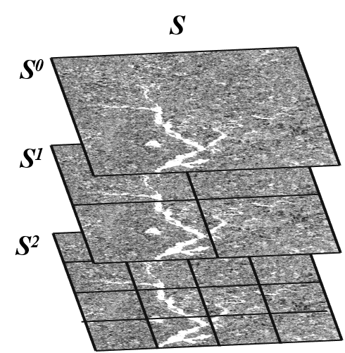
Figure 4: Example of a quad-tree tailing with three levels.
The hierarchical tiling consists of iteratively decomposing image regions into four equally sized quadrants, the so-called sub-quadrants. In the hierarchical approach - a schematic representation of which is shown in Figure 4 - each quadrant or sub-quadrant is related to a given node in the tree and has exactly four children or no children at all. The latter is referred to as a ‘leaf node’. Each node is associated with a specific region of the image Laferte et al (2000). Let I be an image and SnodesS_{nodes}Snodes the ensemble of tree nodes. A node in the i-th tree level is denoted Sji∈SnodesS_j^i∈S_{nodes}Sji∈Snodes, where S0S^0S0 is the root node, associated with the tile that completely encloses I, and SNS^NSN is the ensemble of nodes in the lowest level having the smallest tile size. The tile related to Sji∈SnodesS_j^i∈S_{nodes}Sji∈Snodes is split into four tiles in the next lower level (i+1). It is itself one of the four quadrants of a tile in the level above (i-1). Thus, the resulting quad-tree decomposition can be expressed as:

where I[Sji]I[S_j^i]I[Sji] is the portion of the image related to node Sji∈SnodesS_j^i∈S_{nodes}Sji∈Snodes and U represents the Union operator (see Figure 4).
The lowest level of the quad-tree decomposition is fixed based on the minimum tile size that still guarantees statistical representativeness. A tile is selected based on three conditions (C1, C2, C3):
- C1: The tile histogram, h(I[Sji])h(I[S_j^i])h(I[Sji]) , is clearly bimodal;
- C2: The two populations represented in h(I[Sji])h(I[S_j^i])h(I[Sji]) are normally distributed;
- C3: Each population in h(I[Sji])h(I[S_j^i])h(I[Sji]) is present at a frequency of at least 10% of the frequency of the other class Bazi et al. (2007).
It is hypothesized that each h(I[Sji])h(I[S_j^i])h(I[Sji]) is a sum of two Gaussian curves, i.e.

where A1A_1A1 and A2A_2A2 are scale factors set to the maxima of the two curves; μ1μ_1μ1 and μ2μ_2μ2 are the distribution means; σ1σ_1σ1 and σ2σ_2σ2 are the distribution standard deviations; yyy is the measurement and hf(y)h_f (y)hf(y) is the fitted histogram.
In order to estimate the parameters of the two Gaussian curves in (Eq. 4 2), G1(y)G_1 (y)G1(y) and G2(y)G_2 (y)G2(y), which in combination compose the histogram, the Levenberg-Marquardt algorithm is applied. It solves the nonlinear least squares problems by combining the steepest descent and inverse-Hessian function fitting methods Marquardt et al. (1963). Nonlinear least squares methods involve an iterative optimization of parameter values to reduce the sum of the squares of the errors between a fitting function and histogram values. Iterations are carried out until three consecutive repetitions fail to change the chi-squared value by more than a specified tolerance amount, or until a maximum number of iterations has been reached. The initial guess of the parameter values should be as close as possible to the actual values, otherwise the solution may not converge. The Otsu approach Otsu et al. (1979) is used for retrieving the first guess values. Given the Otsu-based thresholds, τOtsuτ_{Otsu}τOtsu for h(y)h(y)h(y), the first guess values (denoted by the superscript 0) of the parameters of the two Gaussian distributions defined in (2) can be derived as:

When all distributions have been fitted, the Ashman D (AD) coefficient Ashman et al. (1994), the Bhattacharyya Coefficient (BC) Aherne et al. (1998) and the Surface Ratio (SR) of the two classes on image III are used for evaluating the bimodality of the histogram, the Gaussianity of each class distribution and the balance of each class in the image, respectively.
The AD coefficient quantifies how well two Gaussian distributions are separated, by considering the distance between their mean values and their dispersions, i.e. standard deviations, and it is expressed as:

For a mixture of two Gaussian distributions, AD > 2 is required for a clear separation of the distributions Ashman et al. (1994). Consequently, the condition C1 for selecting or not a tile is defined as:

The BC evaluates the similarity of two distributions. It is used here to verify if hf(y)h_f (y)hf(y) is a good approximation of h(y)h(y)h(y), meaning that the hypothesis of having two Gaussian distributions is verified and defined as:

where k is the corresponding bin of the two discrete histograms. In the case of two almost identical histograms, the BC approaches 1 Aherne et al. (1998). As an approximation, we assume that BC has to be higher than .99 for a good fitting. Consequently, the condition C2 for selecting or not a tile is computed as:

Once all distributions have been parameterized, the verification of the remaining condition C3 is straightforward. To do so, the SR between the smallest and the largest class is computed, i.e.

Considering that C3 stipulates that the smaller population should represent at least 10% of the other one, condition C3 becomes:

Technically speaking, the tiles of the entire tree are scanned starting from S0 until SN. Any node (and the associated tile) that fulfils the conditions C1(I[Sji])=1C1(I[S_j^i])=1C1(I[Sji])=1 and C2(I[Sji])=1C2(I[S_j^i])=1C2(I[Sji])=1 and C3(I[Sji])=1C3(I[S_j^i])=1C3(I[Sji])=1 (see Eq. 4 8 to Eq. 4 11) is finally selected and its children, tiles at levels with higher i, are no longer considered as possible tile candidates. These processing steps result in a binary map, henceforth named Bimodal Mask (BM). BM includes regions in I where the distinctive populations, G1G_1G1 and G2G_2G2, are present with a sufficient number of pixels and where their respective distribution functions are clearly identifiable with more balanced prior probabilities.
At this point, all subtiles fulfilling the three conditions C1, C2 and C3 are selected. Hence, the histogram of all the pixels enclosed by the selected tiles, i.e. where BM=1, has to be clearly bimodal. This histogram, h(I[whereBM=1])h(I[where BM=1])h(I[whereBM=1]), is used to estimate the Gaussian distributions of the two classes of interest, hereafter named G1BM(y)G_1^{BM} (y)G1BM(y) and G2BM(y)G_2^{BM} (y)G2BM(y). To do so, the Levenberg-Marquardt algorithm is re-applied to fit two Gaussian curves on the histogram pixel values obtained from the union of all selected tiles. Starting from the two derived Gaussian distributions, the objective is to select the threshold for separating the two classes.
The algorithm needs to handle different type of flood events, from those lasting few days up to those lasting weeks, as the case of monsoon events. As a consequence, the algorithm assumes that the floodwater extent in the newly acquired S1 scene, It0S1I_{t0}^{S1}It0S1, i) increases or ii) only decreases. Regarding the case (i), increase, the algorithm assumes that there are also areas where the water extent can recede. These two different floodwater evolutions are handled subsequentially: the condition (i) is checked firstly, if it is satisfied the newly floodwater is mapped, if not it is checked the condition (ii) and the receding water is removed from the previous floodwater map. If both conditions are not satisfied means that the floodwater states in It0S1I_{t0}^{S1}It0S1 does not change with respect to the previous acquired scene, It−1S1I_{t-1}^{S1}It−1S1.
i) First, the image difference is computed between It0S1I_{t0}^{S1}It0S1 and It−1S1I_{t-1}^{S1}It−1S1, i.e. IDS1=It0S1−It−1S1I_{D}^{S1}= I_{t0}^{S1} - I_{t-1}^{S1}IDS1=It0S1−It−1S1, then HSBA is applied in parallel to I_t0^S1 and I_D^S1 in order to select tiles that show a bimodality behaviour on both images, guaranteeing that It0S1I_{t0}^{S1}It0S1 is affected by floodwater and I_D^S1 is characterized by a class representative of a decrease of backscattering with respect to It−1S1I_{t-1}^{S1}It−1S1. The final BM is used to estimate PDFs of water and non-water, PDF(W) and PDF(NW), in It0S1I_{t0}^{S1}It0S1 and change and non-change in IDS1I_{D}^{S1}IDS1, PDF(C) and PDF(NC). Before to estimate the four PDFs the permanent water layer (from Copernicus DEM or Permanent water from GFM) is removed in order to have PDFs more representative of floodwater pixels in both It0S1I_{t0}^{S1}It0S1 and IDS1I_{D}^{S1}IDS1. All estimated PDFs are used to apply a 2D region growing, It0S1I_{t0}^{S1}It0S1 and IDS1I_{D}^{S1}IDS1, where the thresholds for seeds and to stop the region growing are defined as:
Seeds: Pixels whose posterior probability of water class p(W│σ0)≥0.7p(W│σ^0 )≥0.7p(W│σ0)≥0.7 and posterior probability of change class p(C│∆σ0)≥0.7p(C│∆σ^0 )≥0.7p(C│∆σ0)≥0.7 are selected as seeds for region growing.
Stop growing: Pixels with$ 0.3<p(W│σ0)<0.70.3< p(W│σ^0 )<0.70.3<p(W│σ0)<0.7 and 0.3<p(C│∆σ0)<0.70.3< p(C│∆σ^0 )<0.70.3<p(C│∆σ0)<0.7 are subject to region growing. The stop growing threshold pair (σstop0,∆σstop0)(σ_{stop}^0,∆σ_{stop}^0)(σstop0,∆σstop0) is the one minimizing the root-mean-squared-error (RMSE) between G1BM(y)G_1^{BM} (y)G1BM(y) and the histogram resulting from region growing hrgBM(yseed,yrg)h_{rg}^{BM} (y_{seed},y_{rg} )hrgBM(yseed,yrg).
p(W│σ0)p(W│σ^0 )p(W│σ0) and p(C│∆σ0)p(C│∆σ^0 )p(C│∆σ0) are inferenced via the Bayes theorem:

Where p(σ0)p(σ^0 )p(σ0) is the marginal distribution of backscatter values in It0S1I_{t0}^{S1}It0S1, p(σ0│W)p(σ^0│W)p(σ0│W) and p(σ0│NW)p(σ^0│NW)p(σ0│NW) are conditional probabilities of water and non-water classes, respectively, p(W)p(W)p(W) and p(NW)p(NW)p(NW) are prior probabilities of water and non-water classes, both are set to 0.5. Similarly, p(∆σ0)p(∆σ^0)p(∆σ0) is the marginal distribution of backscatter difference values in IDS1I_D^{S1}IDS1, p(∆σ0│C)p(∆σ^0│C)p(∆σ0│C) and p(∆σ0│NC)p(∆σ^0│NC)p(∆σ0│NC) are conditional probabilities of change and non-change classes, respectively, p(C)p(C)p(C) and p(NC)p(NC)p(NC) are prior probabilities of water and non-water classes, both are set to 0.5.
From the selected seeds are removed all those that occur in areas masked out by the HAND mask in order to avoid that false alarms in not prone flood areas could spread in plausible areas. The newly detected flooded areas are used to update the previous floodwater map.
The algorithm checks also areas where floodwater could have receded with respect to the previous acquisition. To do this, P(W)P(W)P(W) and P(NW)P(NW)P(NW) are used to apply a 1D region growing to map water on It0S1I_{t0}^{S1}It0S1. The resulting water map is compared with the previous floodwater map and only those pixels that belonging to water in both maps are mapped as floodwater in the new map.
The procedure above mentioned can have a dual role, to map new floodwater and at the same time to check the occurrence of a flood event which is assured by the selection or not of tiles of BM. If BM is an empty mask means that there is not a new flood event in the region or that the flood already ongoing at the time t-1 is only receding. In this latter case, the step ii is applied.
ii) In this case HSBA is applied only to It0S1I_{t0}^{S1}It0S1 to fit P(W)P(W)P(W) and P(NW)P(NW)P(NW), which are subsequentially used for the 1D region growing on It0S1I_{t0}^{S1}It0S1 to map water. The resulting water map is compared with the previous floodwater map and only those pixels that belonging to water in both maps are mapped as floodwater in the new map.
The exclusion layer, the HAND mask and the ocean mask from the Copernicus DEM are applied to mask out all pixels which are not part of flood prone areas.
¶ Flood mapping algorithm 2 (DLR)
GFM flood mapping algorithm 2 requires a full Sentinel-1 scene as the main input and further exploits three ancillary raster datasets: a digital elevation model (DEM), areas not prone to flooding and reference water. Initial descriptions of the algorithm were published by Martinis et al. (2015) and Twele et al. (2016).
The algorithm applies a parametric tile-based thresholding procedure by labelling all pixels with a backscatter value lower than a threshold to the class water. The threshold is computed on a smaller, limited number of subsets of the SAR scene and applied to the entire scene. Subsets used to define the threshold are selected for based on their backscatter values, which should consist of both low backscatter and a strong variation in therein.
In a first step, a bi-level quadtree structure is generated with the division of a SAR scene into N_tiles quadratic non-overlapping subsets (parent tiles) of defined size c2 on level S+ (parent tiles). Each parent tile is represented by four quadratic child objects of size (c/2)²(c/2)²(c/2)² on level S- (Figure 5). The variable c is empirically set to 200 pixels. A limited number of tiles are selected out of NtilesN_{tiles}Ntiles, based on the probability that the tiles contain a bi-modal mixture distribution of the water and non-water classes.
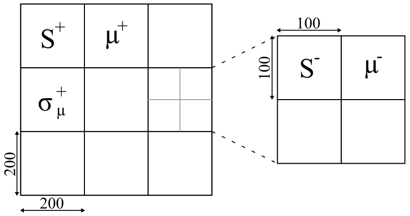
Figure 5: The SAR scene is tiled into N quadratic non-overlapping tiles S+. µ+ is the mean backscatter value of one tile S+. Each tile S+ is further divided into 4 sub tiles S-. µ-^ is the mean backscatter value of one sub tile S-.
In rare cases, a parent tile intersects with the edge of a SAR scene, which results in dimensions that are smaller than the pre-defined size c2c^2c2. Consequently, these tiles are excluded from the threshold computation (Figure 6). Furthermore, due to the near-cross polar orbits of Sentinel-1, the along track direction forms an angle of ~10° with respect to the north-south direction, which can result in parent tiles with variable amounts of no-data content. If no-data comprises of > 50 % of the overall data content, the tile is also excluded from the threshold computation (Figure 6).
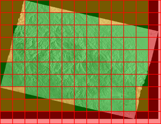
Figure 6: Red tiles intersect with the edge of the SAR scene. Orange tiles have less than 50 % valid data content. Only green tiles are valid and considered for the threshold computation.
A parent tile S+ must fulfil two conditions to be selected as a representative subset (Eq. 4-16):
- S+ must have a lower mean than the global mean of the SAR scene; and
- S+ must have a high standard deviation, which is computed on all S-.

Considering the first condition, for each parent tile S+, the algorithm detects the mean backscatter value µ+ of S+, which must be lower than the mean backscatter value µglobal of the entire SAR scene (Eq. 4 17). We conduct this step to select for tiles with low backscatter content that are likely to contain water features.

Considering the second condition, for each of the four child tiles S- belonging to a parent tile S+, the algorithm detects the mean backscatter value µ- of S-. In a further step, we compute the standard deviation σµ+ of these four mean backscatter values [µ1−,µ2−,µ3−,µ4−][µ_1^-, µ_2^-, µ_3^-, µ_4^-][µ1−,µ2−,µ3−,µ4−] (Eq. 4 18). We conduct this step to characterize the backscatter distribution of each parent tile S+.

We assume that tiles with a low mean backscatter µ+ and a high standard deviation σµ+σ_µ^+σµ+ show a bimodal backscatter distribution and are likely to contain both water and non-water features. In order to fulfil condition 2, we select a parent tile S+ with a standard deviation σµ+σ_µ^+σµ+ that is as high as possible. When investigating σµ+σ_µ^+σµ+ of a specific tile and bringing it into relation to other tiles, we require σµ+σ_µ^+σµ+ to be greater or equal to the mean μσμ+μ_{σ_μ^+}μσμ+ of all standard deviations σµ+σ_µ^+σµ+ (Eq. 4 19), as well as two times the standard deviation σσμ+σ_{σ_μ^+}σσμ+ of all standard deviations σµ+σ_µ^+σµ+ (Eq. 4 20). Figure 7 depicts a graphical representation of the concept. In Figure 7, plotting all standard deviations σµ+σ_µ^+σµ++ into a gaussian distribution, a standard deviation σµ+ that is greater or equal to the distribution’s mean would still leave too many parent tiles S+, i.e. the majority of the tiles may not show a bimodal backscatter distribution. By restricting σµ+σ_µ^+σµ+ to even exceed the mean and one standard deviation we focus on a small number of parent tiles where the standard deviation σµ+σ_µ^+σµ+ is high enough to ensure bimodal backscatter distributions.
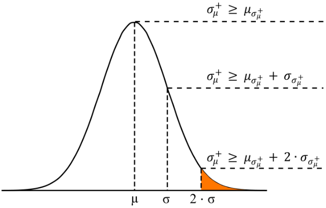
Figure 7: The standard deviation σµ+ in relation to further statistical parameters. (See text for details).

Applying Eq. 4-16 to all valid parent tiles selects suitable tiles for further threshold computation. If the count of suitable parent tiles S+ is less than or equal to 10, Eq. 4-16 is re-applied with x = 1.28, thus the range of allowed standard deviations increases with the inclusion of more parent tiles into the selection. If the count of suitable parent tiles S+ exceeds 10, we assume that there is a statistically sound basis of representative tiles and use the five tiles with the highest standard deviation σµ+σ_µ^+σµ+, i.e. the highest standard deviation of the means of the corresponding child tiles for further threshold computation.
Each of the five final parent tiles should have a bimodal backscatter distribution, which is likely to contain a valid water-land-boundary (Figure 8). We apply the thresholding algorithm of Kittler & Illingworth (1986) to each of the five parent tiles. The algorithm is an iterative, cost-minimization approach, where the histogram is split into two classes with a threshold that identifies the class boundary. The optimal threshold τ separates both classes with minimum effort (Figure 8). In Figure 8, if selecting a pure land tile (a1), the corresponding histogram (a2) is unimodal. If selecting a tile with both low and high backscatter values (b1), the corresponding histogram (b2) is bimodal and we assume depicting a water-land-boundary. If applying a threshold to the histogram b2, both classes can be separated giving the class water in the left part.
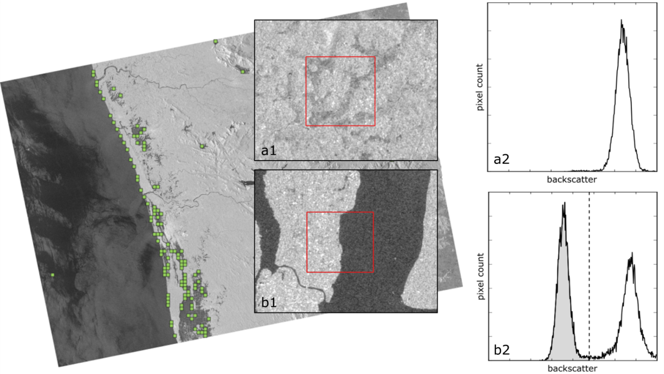
Figure 8: Selecting suitable subsets (green) from the SAR scene. (See text for details).
The final threshold separating the water and land classes is the mean of the thresholds of the parent tiles τ+ (Eq. 4-21).

We further compute the mean of the water class µwater according to Kittler & Illingworth (1986), which describes the geometric centroid of the separated class (Eq. 4 22, with μi(σ0)μ_i (σ^0)μi(σ0) as a function of the SAR backscatter value σ0σ^0σ0. h(g)h(g)h(g) is the SAR backscatter histogram, and g are the histogram bins g. Pi(σ0)P_i (σ^0)Pi(σ0) represents the summed-up histogram h(g), up to the class-separating threshold (Eq. 4 23).
As the thresholding algorithm is an iterative process, a and b denote updatable greyscale values (i.e. SAR backscatter) within the value range.

An average of all “water class centers” µwaterµ{water}µwater is also computed with the same method as the mean threshold τ for the entire SAR scene.
Applying this threshold to the entire SAR scene returns an initial basis for water detection.
¶ Flood mapping algorithm 3 (TUW)
GFM flood mapping algorithm 3 Bauer-Marschallinger et al, (in review) requires three inputs: the SAR scene to be processed, a projected local incidence (PLIA) layer, and the corresponding parameters of the harmonic model. Based on these inputs, the probability of a pixel belonging to the flood or non-flood class is defined. For this purpose the a-priori flood and non-flood probability density function (PDF) is required. For the values of an incoming Sentinel-1 image, the most likely class is selected by the use of the Bayes decision rule. The algorithm’s output consists of a flood extent map and the corresponding estimation of the classification’s uncertainty.
Flood backscatter probability density function:
Due to specular reflections of the radar pulses by water surfaces, the received backscatter intensities by the sensor are significantly lower compared to most other land cover types. Consequently, a temporarily inundated surface is detectable by a significant drop in its backscatter relative to the time series. In order to ensure the drop results from inundation and no other effect, a detailed statistical knowledge of the backscatter behaviour over water surfaces is required. The proposed concept is the definition of the flood backscatter probability density function p(σ0│F)p(σ^0│F)p(σ0│F) for any given incidence angle θ. It is assumed that the p(σ0│F)p(σ^0│F)p(σ0│F) is a normal distribution and can be parametrized by the statistical value-pair of mean and a standard deviation.
Therefore, various backscatter observations (further referred to as σW,θ0σ_{W,θ}^0σW,θ0) and their respective incidence angles were collected over oceans and inland waters from the Sentinel-1 datacube. By sorting the water backscatter collection σW,θ0σ_{W,θ}^0σW,θ0 along the incidence angle (Figure 9), the expected indirect relation of water backscatter values and incidence angles can be confirmed.
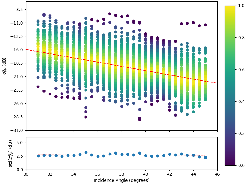
Figure 9: Scatterplot of water backscatter observations grouped by 0.5 degree bins (top). Standard deviation of these bins (bottom).
The mean backscatter value at a specific incidence angle can be derived by the use of a linear regression. The corresponding gradient was found to be 0.394 (red line in upper Figure 9). In order to analyse the standard deviation at a specific incidence angle, the water backscatter values were grouped into 0.5 degree bins. As shown in the bottom of Figure 9, the gradient of the standard deviation per bin is small with 0.008. Therefore, homoscedasticity is assumed and the total standard deviation is calculated by the square root of the sum of squared estimate of errors (SSE), normalised with respect to the number of data points (NpointsN_{points}Npoints). To summarize, the flood backscatter probability density function p(σ0│F)p(σ^0│F)p(σ0│F) is defined by:

Non-flood probability density function:
In order to model the normal, non-flooded circumstances, we propose the use of the harmonic model (details given in Section 0). The harmonic model allows retrieving an expected backscatter value σt,r0^\hat{σ_{t,r}^{0}}σt,r0^ for any day of the year tdayt_{day}tday and a specific relative orbit rrr. Therefore, the backscatter’s seasonality is modelled by defining the pixel’s harmonic parameters (CiC_iCi, SiS_iSi and σ0ˉ\bar{σ_0}σ0ˉ) based on its backscatter time-series σr0σ_r^0σr0 (see Eq. 3 1). Furthermore, this model is taken as base of the non-flood probability density function p(σ0│NF)p(σ^0│NF)p(σ0│NF),which is assumed to be a normal distribution. The mean backscatter value is set to the expected backscatter of the harmonic model σt,r0^\hat{σ_{t,r}^{0}}σt,r0^. As mentioned in Section 3.1.3, in addition to the harmonic parameters the standard deviation s of the harmonic model is used as an input for the algorithm and standard deviation of the PDF.

A redundancy criterion is introduced to reduce the possibility of ill-fitting harmonic parameters (especially for sparse data sets). This criterion makes use of the NOBS layer (introduced in Section 3.1.3) which indicates the number of valid observations used for the estimation of the harmonic parameters. Given the requisite 2k + 1 samples for a unique solution to the harmonic equation, redundancy criteria is applied as a multiple of this number. Since the pixels which do not match the redundancy criteria are excluded from the flood mapping procedure, one needs to find a balance between number of excluded pixels and introduced noise. Based on initial tests, a redundancy value of 4x, e.g. 28 samples per pixel stack, can be set in order to minimizing noise , specifically at edges where sparse samples might be present.
Bayesian Decision:
With the per-pixel knowledge of the relative orbit rrr, the day of year t_day and the incidence angle θ, one is able to define the flood backscatter probability density function p(σ0│F)p(σ^0│F)p(σ0│F) and the non-flood probability density function p(σ0│NF)p(σ^0│NF)p(σ0│NF) for each pixel. By using these PDF the belonging of the incoming Sentinel-1 image to either the flood (F) or non-flood (NF) class can be determined on a pixel-level. Therefore, the Bayes decision rule makes use of the class’ posterior probability:

Where P(F)P(F)P(F) and P(NF)P(NF)P(NF) are called prior probabilities and represent the prior knowledge of the pixel’s belonging to a certain class. Since no prior information is available, it is set to equal weight (0.5). The evidence p(σ0)p(σ^0)p(σ0) scales the posterior probabilities between 0 and 1 and is defined by:

By selecting the class (c)(c)(c), featuring the maximum posterior probability the Bayes decision rule selects the most likely class. Details can be seen within Eq. 4 31, where the class set fj={f1,f2}={F,NF}f_j= \{f_1,f_2\}=\{F,NF\}fj={f1,f2}={F,NF} includes the flood (F) and non-flood (NF) classes. Figure 10 shows the decision step graphically. Finally, each pixel’s belonging to the flood (F) class generates the preliminary binary flood extent map.

Uncertainty Values:
The algorithm provides the ability to quantify the uncertainty of the classification by the use of the conditional error P(error│σ0)P(error│σ^0)P(error│σ0). This measure is the posterior probability of the less probable class (i.e. the class not selected as flood), is defined between 0.0 and 0.5, and directly quantifies the uncertainty of the classification decision.
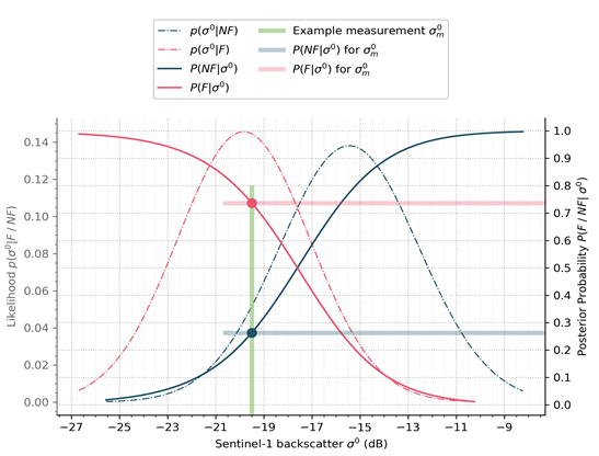
Figure 10: Exemplary Bayes flood mapping process for a single pixel. Including the probability density function and posterior probability of the flood and non-flood class. In this case the backscatter value of -19.5dB would be classified as flood.
Low-Sensitivity Masking:
For improving the reliability of Algorithm 3 in (non-supervised) operations, we introduce a set of routines to exclude locations where our statistical model does not allow a robust decision between flood and non-flood condition. Consequently, the following masks (PLIA, distributions conflicts, outlier, and high uncertainty) are applied on the preliminary flood extent map obtained from the Bayes decision. Figure 11 shows an exemplary overview of the applied low sensitivity masks over Greece.
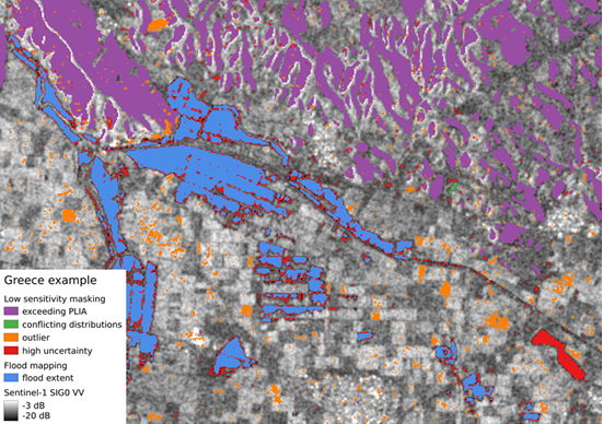
Figure 11: Example of low sensitivity masking in Algorithm 3 over Greece.
Flat areas are observed by Sentinel-1’s IW mode within a viewing angle between 29° and 46°. Since (flat) water surfaces fall per definition into this PLIA-interval, the collection of water backscatter samples (described above) was limited accordingly. To extend the flood mapping capabilities to e.g. onsets of hills, the allowed range is relaxed to 27° to 48°. In order to pre-filter the pixels which feature an exceeding PLIA-value (θ), the following PLIA mask is introduced:

Our algorithm detects flood if a normally non-flooded pixel is temporary inundated which implies the pixel features a higher backscatter than a respective water surface. Putting it into context, the non-flooded PDF needs to be overall higher than the flood PDF. Typical locations where this requirement is not fulfilled are e.g. permanent water bodies, asphalt surfaces, salt panes, or very dry sand- and bedrock-areas. In order to exclude these cases of conflicting distributions, a pixel is masked if the mean of the non-flood PDF is lower than the mean of the flood PDF raised by half the standard deviation of the water PDF:

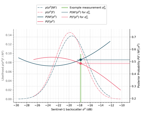
Figure 12: Example of a conflicting distribution situation.
Besides the above mentioned all-season low backscatter situations (e.g. permanent water bodies, water look-alikes, etc.), the backscatter could be low for some seasons of the year only (e.g. rainy season, snow melting, etc.). An example of a conflicting constellation from the flood and non-flood PDFs is given in Figure 12. The consideration of such seasonal effects is one of the main features of the used harmonic model approach (details given in 3.1.3). In that perspective, if the used input observations show regularly low backscatter within a certain season, the corresponding expected DOY backscatter represents this for the flood mapping unfavourable behaviour. Figure 13 shows an example over France (near the city of Angers) in January 2022, where the expected DOY backscatter (a) shows a large area of low backscatter pixels, which may be related to seasonal inundation. Indeed, similar inundations can be observed in other recent years (b – e) as well. The harmonic model was trained in the current version by data from the years 2019 – 2020, and hence appear to reflect the local dynamics in that perspective.
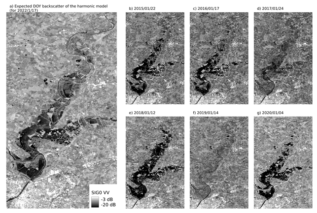
Figure 13: Example of the expected DOY backscatter compared to the Sentinel-1 observations from recent years (near the city of Angers, France).
Our statistical model is trained to provide robust decisions on normal flood conditions. Therefore, a meaningful Bayes decision cannot be provided in case of the input Sentinel-1 backscatter value (σ0σ^0σ0) not being represented by the flood or non-flood PDF. These extreme values could arise due to a statistical outlier for example and is masked by the following definition. Since it is assumed that the lower outliers of the flood PDF can still be classified as flooded, only higher outliers of the flooded PDF are considered within the masking. An example of an outlier observation is given in Figure 14.

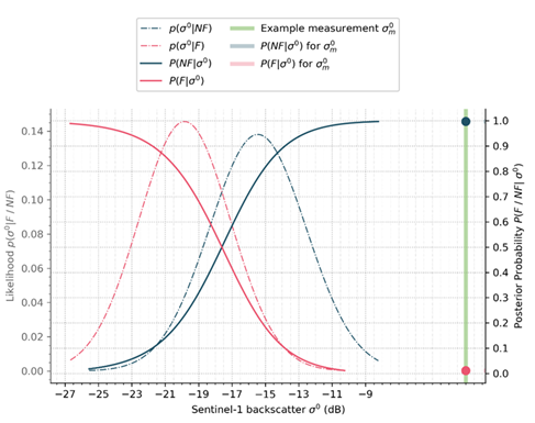
Figure 14: Example of a detected outlier measurement.
As the uncertainty (from the Bayes decision, details are given in Section 4.5.4) provides a measure for the confidence of the decision between flood and non-flood, it is used to limit the classification to certain decisions only. Therefore, we introduce a dedicated mask for high uncertainties which excludes pixels with uncertainties higher than 0.2:

An example of an uncertain decision is given in Figure 15. One can see that the incoming measurement is nearly equally probable to be assigned to one of the two classes (flooded and non-flooded).
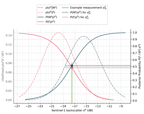
Figure 15: Example of pixel classification which shows a high uncertainty.
Morphological post-processing:
Due to the coherent nature of the radar signal, a single-time Sentinel-1 observation is in general affected by multiplicative noise (known as speckle). The random signal variation could lead to single pixels that feature a lower backscatter and could be confused with flood conditions. In order to reduce the influence of noise on the final flood extent map, a median filter of kernel size 5 is applied. This constitutes the final step and the result represents the flood extent and uncertainty output of algorithm 3.
¶ Ensemble flood mapping algorithm
The GFM ensemble flood mapping algorithm combines the flood and likelihood results produced with all three individual flood mapping algorithms. The output is entirely pixel-based. A consensus decision of all algorithms, based on majority voting, determines if a pixel is marked as flooded or as non-flooded. To generate the combined product, each pixel is attributed with the ratio of the number of classifications as flooded to the number of algorithms that were applied. The value range is [0, 1] with:
Table 5: Degree of consensus to determine if a pixel is classified as flooded in the ensemble flood map

A value of 1.0 means that all three algorithms agreed on its classification as being flooded. A pixel is classified as flooded if it was classified as flooded by at least two algorithms.
The ensemble algorithm accepts Geotiff files for both the classification and uncertainty layers of each algorithm. The algorithm checks if all layers can be loaded. If a flood layer from one of the algorithms cannot be loaded, it is likely that the particular algorithm failed to produce a result. The number of algorithms applied equals to the number of flood layers that were loaded successfully, such that if one layer failed to load, the number of algorithms applied is 2.
Each flood result from the algorithms is given between 0 and 1. If two algorithm results could be loaded and both algorithms agreed on a pixel as flooded, the final pixel would have a value 1.0. If two of the three algorithms that could be loaded classified a pixel as flooded, the resultant ratio calculated with Eq. 9 is 0.66. This exemplifies how the majority decision is applied to classify a given pixel as flooded.
The final likelihood layer is generated as the arithmetic mean at each pixelwise location calculated with all likelihood layers provided by each of the algorithms. The term likelihood represents the classification accuracy of a given flood pixel. Likelihood values lie in the interval [0, 100], where values toward 0 represents lower confidence and values toward 100 represents higher confidence of flood classification accuracy. A likelihood value of 50 separates both classes where non-flood pixels necessarily show likelihood values in the interval [0, 49] and flood pixels show likelihood values in the interval [50, 100]. The classification confidence of the respective class increases with likelihood values propagating to the lowest or highest class boundary. Non-flood likelihoods propagate towards 0 if the non-flood confidence is to increase. In contrast to that flood likelihoods propagate towards 100 if the flood confidence is to increase.
As the TUW algorithm produces uncertainty values, TUW uncertainties have to be flipped so that low uncertainty values propagating towards 0 are remapped to high likelihood values propagating towards 100 and vice versa.
A series of potential cases are presented to illustrate how the ensemble algorithm behaves.
Case 1: all algorithms produce inputs with full consent
When all three flood algorithms return the same classification, the ensemble reflects this complete agreement. The final likelihood layer is the pixelwise mean of inputs from all three algorithm likelihood layers.
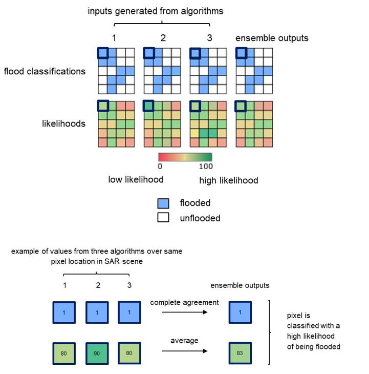
Figure 16: An example of full consent (complete agreement) among all three algorithms and also resulted in a given pixel being classified with a higher likelihood of being flooded.
Case 2: all algorithms produce inputs with majority consent
This is a variation of the usual case where all three algorithms produce inputs to the ensemble computation. If two of three algorithms agree that a pixel classification, the classification of the third algorithm is overruled. The likelihood result is the mean of all three likelihoods.
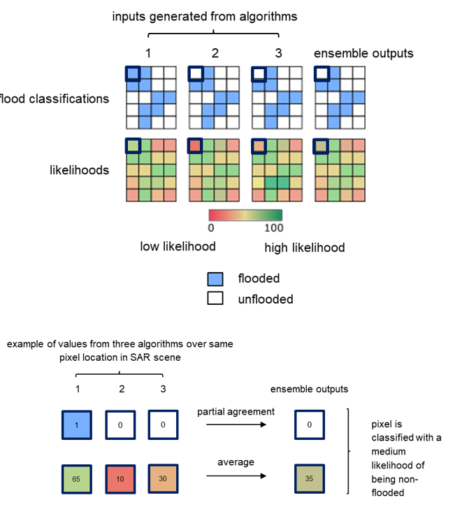
Figure 17: An example of majority consent (partial agreement) among the three algorithms and resulted in a given pixel being classified with a medium likelihood of being non-flooded.
Case 3: inputs from a single algorithm only
There may be cases where certain algorithms fail to produce inputs for the ensemble computation. However, since the ensemble algorithm requires the availability of inputs from at least 2 algorithms, if only one provides results, an empty raster is generated and all pixels are assigned lowest likelihood value of 0.

Figure 18: An example of classification and likelihood inputs being generated by a single algorithm only. Since the ensemble requires inputs from at least 2 algorithms, an empty flood classification raster is generated with the lowest likelihood of 0 assigned to each pixel.
Case 4: inputs from two algorithms only
In the unusual case that one algorithm fails to produce classification and likelihood inputs, the other two remaining algorithms decide on the flood classification For pixels where there is an agreement between the two algorithms (Case 4A), the common classification is forwarded to the final result. This application is consistent with majority voting, which is the basis for the ensemble approach. For pixels where there is disagreement on the classification (Case 4B), i.e. one algorithm classified a given pixel as flooded while the other classified the same pixel as non-flooded, the pixel is assigned with the classification result that shows the highest confidence. The highest confidence is defined as the arithmetic distance to the basic likelihood interval boundaries [0, 100]. The likelihood value 50 has the greatest arithmetic distance.
In case of a split decision, the algorithm with the higher class confidence (greater distance from likelihood 50) overrules the detection from the algorithm with the lower class confidence (Case 4B). If both algorithms disagree on the flood classification but are equally confident in the respective class, the ensemble algorithm favours the flood detection over the non-flood detection (Case 4C).
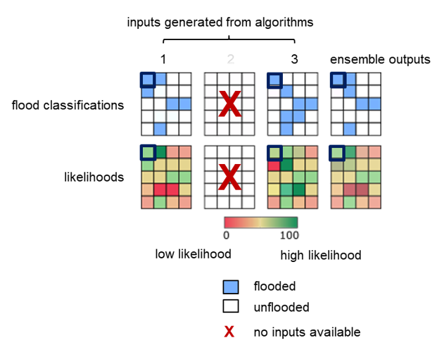
Case 4A: both algorithms agree on classification and have different likelihoods
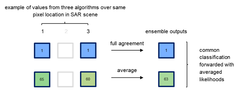
Case 4B: algorithms disagree on classification
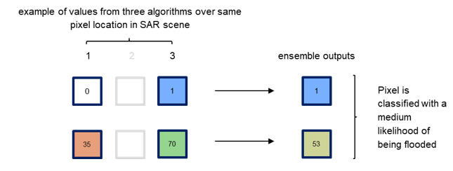
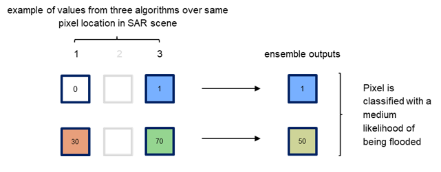
Case 4C: algorithms disagree on classification and have equally strong likelihoods
Figure 19: Examples of three cases when only two algorithms produce inputs, where there is agreement (Case 4A), disagreement with different likelihoods (Case 4B) and equally strong likelihoods (Case 4C) on the classification, respectively.
We apply a region size dependant correction of the ensemble flood pixels and remove any flood pixel that forms a coherent region with its 8 neighbours and is less than a pre-defined blob size of 60. The indices of the removed flood pixels are applied to the likelihood layer so both layers show a consistent handling of valid pixels. As non-flood pixels can have a maximum likelihood of only 49, we correct the likelihood value of pixels that were changed due to their blob size. Pixels that were corrected had a likelihood value of at least 50 (denoting flood) and are now assigned with a likelihood value of 49, i.e. the highest likelihood value that is allowed for non-flood pixels.
For all cases, we apply the reference water layer to the final flood and likelihood layers. This layer is comprised of both permanent and seasonal water extents. At any pixel location where there is the flood layer declares flood and the permanent or seasonal reference water layer also declare the presence of water, the pixel value of the flood layer is set to 0, i.e. no flood.
In a final step, we apply an exclusion layer to the flood and likelihood layer, correcting pixels that were misclassified due to radar shadow, permanent low backscatter and urban areas. We also apply the Copernicus Water Body Mask masking out any oceanic area from the flood ensemble classification.
¶ Output layer “S-1 observed water extent”
The GFM product output layer “S-1 observed water extent” identifies the pixels classified as open and calm water based on Sentinel-1 SAR backscatter intensity, and is derived by combining with a logical OR the ensemble flood map obtained with the algorithm described in section 0 and the seasonal and permanent water mask as described in section "4.3 Output layer “S-1 reference water mask". While the floodwater extent is produced using an ensemble approach which use all three algorithms (i.e. LIST, DLR and TUW), the ensemble approach to provide permanent and seasonal water uses only two algorithms (i.e. LIST and DLR). The “S-1 observed water extent” output layer values are described in Table 6.
Table 6: Description of “S-1 observed water extent” output layer values.

¶ Output layer “S-1 reference water mask”
The GFM product output layer “S-1 reference water mask” outlines pixels that are classified as water, both permanent and seasonal, by an ensemble water mapping algorithm and using Sentinel-1 SAR mean backscatter intensity over a certain time period. The permanent water extent mapping is based on the mean backscatter of all Sentinel-1 data from a reference time period of two years. The seasonal reference water mapping uses as input the median backscatter of all Sentinel-1 data from a given month over the same reference time period. As a result, twelve masks are available, one per month, which include information on the permanent and seasonal reference water extent. The application of a permanent water mask is reliable in environments with stable hydrological conditions over the year. In geographic regions with strong hydrological dynamics related to temporal change and variation in space of the water extent (e.g., in areas affected by monsoonal effects) the additional use of a seasonal reference water mask, which considers the usual water extent of the respective time period, is preferable.
Figure 20 shows an example of reference water masks computed over a test area in Myanmar for the time-period 2019-01-01 to 2020-12-31. Seasonality, by means of monthly variations of water body areas, can be depicted and separated from permanent water bodies, which do not show alterations in their extent during the two years reference time-period. In Figure 20, each mask separates permanent water (pixels classified as water during the whole reference time-period) and seasonal water (pixels classified as water during a specific month within the reference time-period).
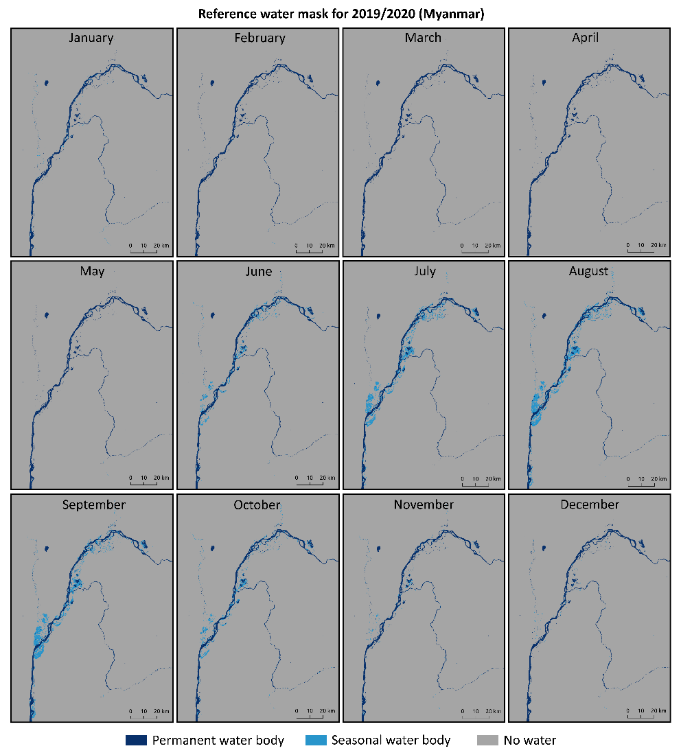
Figure 20: Exemplary reference water masks computed over Myanmar for the time-period 2019-01-01 to 2020-12-31. (See text for details).
The reference water mask product is updated once a year considering the previous two years of observation. This means that for example, the flood monitoring system running in 2021 will rely on the Sentinel-1 reference water mask being extracted from the Sentinel-1 mean backscatter over the reference time period from 2019 and 2020. The reference period of two years is chosen as compromise in order to base the computation on a sufficient number of Sentinel-1 data and to remove long-term hydrologic changes which would be integrated in the reference waters masks if longer time periods would be considered. The Sentinel-1 reference water mask product values are described in the following table.
Table 7: Description of “S-1 reference water mask” output layer values.

¶ Algorithm for generating the S-1 reference water mask
Observed permanent and seasonal water extent mapping is done by an ensemble water mapping algorithm that combines the water and uncertainty results produced with the LIST (see section 3.1.3) and DLR (section 3.1.3) flood algorithms and having as input the mean backscattering value of S1 images available over a two-year time period (for permanent water) or the mean backscattering value of S1 images available over a two-year time period per month (for seasonal water). The results of the single water extent maps are combined into twelve masks, one per month, which include information on the permanent and seasonal reference water extent.
Both LIST and DLR flood algorithms produce a water extent map and associated likelihoods as by-product of the flood detection. In particular, the step ii of the LIST algorithm is used, i.e. the one that map the water extent using a single image and a 1-D region growing as described in the section 0. The TUW algorithm (section 3.1.3) is specifically designed to detect temporary flooded water bodies, does not produce a water extent map and hence is excluded for the more generic task of observed water extent mapping.
Therefore, the ensemble water mapping algorithm follows the same logic as the flood ensemble algorithm (section 3.1.3) but is specifically targeted towards the task of water mapping from two (not three) input sources. This means that a consensus decision of the two algorithms decides if a pixel is marked as water or as no water. To generate the combined product, each pixel is attributed with the ratio of the number of water classifications to the number of algorithms that were applied. A number of 1 would mean that both algorithms agreed on its classification as water. For pixels where they disagree on the classification (one algorithm classified that pixel as water and the other algorithm classified that pixel as no water) the algorithm with the highest likelihood for that classification dictates the result. That means, if the first algorithm is certain that a pixel is water (its likelihood value is high) and the second algorithm declares the pixel as no water with a low classification accuracy (its likelihood value is low), the first algorithm classifying that pixel as water dictates the final result. The likelihood result is the mean of all providing likelihood values for that pixel. If only one algorithm provides results, the final water and uncertainty values equal the results from that particular algorithm.
Finally, for selected tiles where false negatives could be observed (e.g., large lakes with roughened surface that has falsely been classified as land) the Copernicus Water Body Mask is used to correct these. To enforce a consistent land-sea border, a land-sea mask derived from the Copernicus Water Body Mask is applied to all results.
¶ Output layer “Exclusion mask”
The identification of conditions under which the GFM algorithms are deemed reliable is considered essential for an automated global flood monitoring system and is hence integral part during NRT flood detection and final product preparation. The key to a successful SAR-based identification and delineation of water bodies, and in subsequence of flood extents, is the low backscatter signature of water surfaces. Under common conditions, the water surfaces scanned by the SAR show significantly lower backscatter values than the surrounding area, the desired discrimination into water and non-water surfaces can be achieved with high accuracy and reliability. With the inclusion of information generated from time series stored in the datacube, additional discrimination criterions are established, further improving the reliability of the GFM flood extent. Nevertheless, there are several situations when the flood extent delineation is hampered, or even completely impeded, and where an Exclusion Mask is deemed necessary to prevent misclassification.
First, the flood detection is challenged by non-water surfaces that feature low backscatter themselves and would yield false alarms when not treated properly. For instance, very dry or sandy soils, frozen ground, wet snow and flat impervious areas (e.g. smooth tarmac covers as airfields or roads) feature very low backscatter signatures and appear thus as water-look-alikes in SAR imagery. Another common effect in SAR remote sensing is radar shadowing, which appears over strong terrain (especially at the far-range section of the SAR image) as well as in the vicinity of high objects above the ground, like high buildings and along forest borders. Whereas the first can be recognised well with terrain- and observation geometry analysis, the second can only be identified by backscatter time series analysis, considering the global scope of the service (as real Digital Surface Models are only available for some areas).
Second, floods occurring in urban or vegetated areas bear the danger of missed alarms, as co-located flood extents potentially feature high instead of low backscatter. The formation of corner reflectors for the SAR’s microwaves through perpendicular buildings (urban) or plant stems (vegetation) over standing water surfaces leads generally to high backscatter and thus common SAR water mapping approaches fail in detecting water surfaces. Moreover, the detection of water-bodies under densely vegetated canopies is complicated by the absorption and diffuse scattering in the canopy itself, reducing the sensitivity to processes on the ground.
The GFM product output layer “Exclusion Mask” addresses static topography and land cover effects, where the interaction of C-band microwaves with the land surface is in general complex. In several situations, flooded areas cannot be detected by Sentinel-1 C-band SAR over certain land cover types and terrain conditions for physical reasons. We grouped these reasons and defined four types:
Sentinel-1 does not receive sufficiently strong signals from the ground surface to distinguish a flooded from a non-flooded surface. In such a case, we encounter No-Sensitivity to detect water surfaces.
Sentinel-1 senses the ground, but backscatter from the non-flooded surface is in general so low as to be indistinguishable from backscatter from smooth open water. Here we encounter water-look-alikes due to a Low Backscatter signature of the ground.
The Sentinel-1 signals are heavily distorted by terrain effects, effectively enhancing the noise and signal disturbances to such a degree to that it becomes larger than the change in backscatter due to potential flooding. As this problem generally occurs over areas with strong topography, we refer to this with Topographic Distortions.
Sentinel-1 receives no signals from certain regions of the land surface due to Radar Shadows casted by mountains, high vegetation canopies or anthropogenic structures.
Reflecting this grouping of physical and geometrical effects, we generate the Exclusion Mask by combining layers that address the four individual effect groups. With the addition of the no-data values from the expert flood detection algorithm output, it indicates on a binary map the pixel locations where the SAR data could not deliver the necessary information for robust flood delineation. With respect to the complexity of the identified effects, and to potential spatial overlaps and interactions, a combined, single Exclusion Mask that is also easy for the user to interpret, is provided.
¶ Algorithm for generating the Exclusion Mask
The Exclusion Mask is based on offline-generated Sentinel-1 SAR parameters and on auxiliary thematic datasets. It is accessed and subset in NRT and added to the other product layers. The necessary operations are done at the 20m-sampling of the Sentinel-1 preprocessed data cube. In the following, we describe the methods to address the four types of disturbing effects.
¶ Masking of no-sensitivity areas
The no-sensitivity layer delineates all land cover types and areas where Sentinel-1 CSAR is not sensitive to flooding – and in fact any other type of change – of the ground surface. These non-sensitive areas encompass both densely vegetated- and urban areas. In both cases, the loss in sensitivity reflects the fact that the Sentinel-1 signal is dominated by backscatter echoes from other parts of the observed scene.
In the case of vegetation, backscatter from the vegetation canopy increasingly dominates the signals coming from the ground for increasing biomass levels. Given the limited penetration capability of C-band waves, Sentinel-1 becomes essentially insensitive to flooding over high biomass areas such as forests and shrubland with biomass levels larger than 30-50 t/ha Quegan et al., (2000). Backscatter from these high biomass land cover classes is in general rather stable and high, a feature that is often exploited in land cover classification schemes.
To identify the densely vegetated areas, parameters from the Sentinel-1 Global Backscatter Model (S1-GBM) were used, namely the mean backscatter in VV (µVVσ0)(µ_{VV}^{σ^0})(µVVσ0) and VH (µVHσ0)(µ_{VH}^{σ^0})(µVHσ0) polarization, mean cross polarization ratio (µCPRσ0(µ_{CPR}^{σ^0}(µCPRσ0, computed as VV/VH backscatter) and standard deviation in VH polarization (std(σVHσ0)(σ_{VH}^{σ^0})(σVHσ0)). Locally variable thresholds (τ_i) were defined for each parameter to discriminate between the vegetated and not vegetated areas setting the rule that the pixel is classified as dense vegetation in case that the following rules apply:

The thresholds were optimized separately for each continent and varied with northing and vegetation type. The Global Forest Change dataset (Hansen et al., (2013); version 1.8: https://storage.googleapis.com/earthenginepartners-hansen/GFC-2020-v1.8/download.html) was used as a reference dataset for the threshold selection and is used directly as a dense vegetation mask in regions, where the irregular coverage of Sentinel-1 data caused artefacts (e.g. stripes of higher and lower backscatter) in the S1-GBM layers. The global distribution of the thresholds is shown in Figure 21.
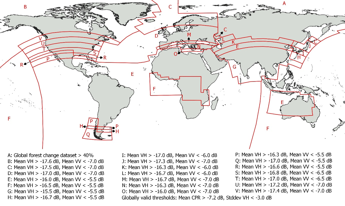
Figure 21: Global distribution of thresholds used to identify densely vegetated areas using S1-GBM and Global Forest Change dataset.
Over urban areas backscatter as measured by C-band SAR sensors is often dominated by comparably few, but very strong echoes received from buildings and other artificial objects (Sauer et al., 2011). The presence of large corner reflectors in form of buildings perpendicular to smooth horizontal ground create an extremely high backscatter signature, often close to saturation. Therefore, in the absence of sufficiently large open spaces between the buildings and urban vegetation, inundation in urban areas is difficult to detect.
To identify the urban areas, GHSL and WSF2015 static urban masks were used. The urban areas were defined as pixels, where (i) the GHS-BUILD value exceeds 30% probability of built up area and (ii) are identified as settlements in WSF2015 urban mask.
Lastly, the dense vegetation mask and urban areas mask were combined into the binary No-sensitivity mask.
¶ Masking of non-water low backscatter areas
There is another situation where Sentinel-1 is not sensitive to the flooding of the ground, but for quite a different reason as for vegetation and urban areas. In this second case, the lack of sensitivity is related to the fact that backscatter from rather smooth surfaces (smooth compared to the 5.5 cm wavelength of Sentinel-1) can be as low as backscatter from a water surface. Smooth non-water surfaces may act similar like water as a specular reflector scattering most energy of the SAR signal in forward direction, leading to very low backscatter values. Examples of such permanently low-backscatter areas are tarmacs (e.g. airports, motorways, etc.) or sandy surfaces (e.g. in riverbanks and deserts). The separation between water and smooth land surfaces based on a single SAR acquisition is hardly feasible. Therefore, the generation of a water look-alike layer with permanent low backscatter is performed based on statistical information from Sentinel-1 time-series data; pixels are masked in case that the occurrence of low backscatter values (below –15 dB) exceeds 70% of all values in the respective time-series.
¶ Masking of topographic distortions
The consideration of information on local topography is essential to flood detection in two ways. There are areas that must be excluded during flood detection due to the geometry of the SAR observation – this is dealt with measures discussed in next subsection.
Then there are areas that shall be excluded from flood detection because of the nature of the phenomenon itself, as floods appear commonly over non-sloped surfaces, in vicinity to streams, rivers, and other permanent water bodies. The latter is addressed by the Height Above Nearest Drainage (HAND) index. The consideration of the HAND index is of vital importance to the reliability of the flood detection algorithms, as SAR signal disturbances over strong topography can be substantial and dominate the surface backscatter signature, and its change over time, leading to otherwise uncontrollable over- and underestimation of flood indications.
Based on the HAND index, a binary exclusion mask (termed ”HAND-EM”) has been calculated to separate flood-prone from non-flood prone areas based on the elevation of each pixel to the nearest water-covered pixel Twele et al., (2016); Chow et al. (2016), which we use as input the Exclusion Mask.
Both binary classes are determined using an appropriate threshold value. Choosing the threshold value too high may lead to misclassifications (i.e. the inclusion of flood-lookalikes in areas much higher than the actual flood surface and drainage network) while a threshold value set too low would eliminate valid parts of the flood surface. The choice of an appropriate threshold is thus critical, and was derived through a series of empirical tests including more than 400 Sentinel-1 and TerraSAR-X datasets of different hydrological and topographical settings Twele et al., (2016).
Due to the global application scope of the GFM Sentinel-1 flood processing chain, a rather conservative threshold value of ≥15 m was finally chosen for defining non-flood prone areas. The HAND-EM has been further shrunk by one pixel using an 8 neighbour function to account for potential geometric inaccuracies between the exclude layer and the radar data.
It must be noted that the Copernicus DEM is not hydrologically conditioned, hence the HAND index cannot be computed on this version of the elevation model.
¶ Masking of Sentinel-1 radar shadows
Radar shadow is a term for unreachable areas by a radar signal, where no information can be gained. Such areas are commonly located in mountainous regions, around high anthropogenic structures, and along forest borders (forest lines). The extent of radar shadows increases with radar range, thus the far range section of a SAR scene is more affected by it. After preprocessing, radar shadow areas have extreme low backscatter values, and are therefore very likely to be confused with water surfaces leading to false alarms in flood detection.
Radar shadows caused by mountains can be rather easily detected by analysing the SAR sensing geometry with respect to a Digital Elevation Model (DEM). This can be computed offline with a geometric observation model of the Sentinel-1 orbits, without using the Sentinel-1 SAR archive.
However, a DEM may only describe the terrain elevation not the surface elevation or may have a too coarse resolution to catch finer details, thus it does not necessarily include anthropogenic structures or forests. The radar signal (at C-band) is mainly reflected at the surface leading to discrepancies with respect to a terrain model. Therefore, a geometric observation model is not applicable for such smaller structures causing radar shadows. For example, shadows on the boundary of a forest as shown in Figure 22 would be missed. Fortunately, we can make use of the fact that radar shadow depends also on the azimuthal looking angle and can be extracted by analysing backscatter from multiple orbits in different orbit pass directions (ascending and descending). Radar shadow areas are characterised by huge differences in backscatter for opposite orbit directions, where one direction is prone to shadowing and the other to double bounce scattering effects causing high backscatter values.
We analyse these differences for orbits of opposite directions, and generate a radar shadow mask for each Sentinel 1 relative orbit number (which feature a very stable viewing geometry): By comparing mean of backscatter at one orbit with mean of backscatter from orbits in the opposite direction, the extent of the orbit specific shadow areas can be estimated.
For a given orbit, pixels will be masked as shadow, when the mean of backscatter at current orbit is less than -15 dB and mean of backscatter from orbits in the opposite direction is higher than -10 dB. (see also Figure 22 below for illustration).
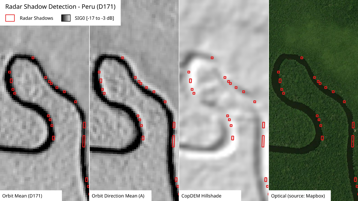
Figure 22: Radar shadow effect on the boundary of forest (columns from left to right): mean backscatter from decending orbit 171, mean backscatter from ascending pass, Copernicus DEM, optical image from Mapbox satellite map.
Because of the new availability of the Copernicus DEM as a digital surface model with an appropriate spatial resolution it could be considered to derive a shadow mask based on a geometric observation model. However, a benchmarking of both outputs is missing, but due to its simplicity, computation time and independency on auxiliary data, preference is given to backscatter differences of opposite orbit directions.
¶ Output layer “Likelihood values”
The GFM product output layer “Likelihood values” provides the estimated likelihood that is associated with the applied GFM flood mapping algorithms, for all areas outside exclusion mask.
¶ Estimation of uncertainty for flood mapping algorithm 1 (LIST)
The likelihood of floodwater classification is characterized by flood probability. In the case (i), both It0S1I_{t0}^{S1}It0S1 andIDS1I_{D}^{S1}IDS1 are used for likelihood estimation, the pixels those have high posterior probability of both water class and change class are likely to be real flooded pixels. The probability of been flooded for a given pixel is defined as the minimum value between p(W│σ0)p(W│σ^0 )p(W│σ0) and p(C│∆σ0)p(C│∆σ^0)p(C│∆σ0):

In the case (ii), only It0S1I_{t0}^{S1}It0S1 is considered for likelihood estimation of flood classification:

As in this case the likelihood is only calculated from the backscatter value in It0S1I_{t0}^{S1}It0S1, false high flood probability can be caused by permanent water and other water look-alike dark areas, these false alarms in binary map has been removed by comparing the resulting flood map with the previous flood map as described above. To reduce these false high probabilities in current likelihood map, for non-flood pixels in the new flood map, their flood probability is the minimum value between p(W│σ0)p(W│σ^0)p(W│σ0) and the value in the latest previous likelihood map.
In both cases of (i) and (ii), the flood probability of pixels located in exclusion layers is set to 0.
¶ Estimation of uncertainty for flood mapping algorithm 2 (DLR)
A fuzzy logic-based approach is applied to measure and to reduce the uncertainty associated with the water classification. Three cases influence the classification likelihood:
The likelihood of a SAR backscatter pixel being classified as water is low if that pixel value is close to the threshold τ.
The likelihood of a SAR backscatter pixel being classified as water is high if the slope at that location is low, since steeper surfaces are unlikely to retain water.
The likelihood of a SAR backscatter pixel being classified as water is high if that pixel forms a coherent area with other neighbouring water pixels and the area is relatively large.
Figure 23 demonstrates the fuzzy logic approach in detail for the first case considering the SAR backscatter likelihood. In Figure 23, the threshold τ of the parent tile is the upper fuzzy value x2 and separates the water and non-water (land) classes. This value represents the boundary of both classes, where the uncertainty of a correct classification is highest. The mean backscatter value of the class water µwaterµ_{water}µwater is associated with a lower fuzzy value. As the majority of water pixels share that backscatter value, the likelihood of a correct classification is high. In fuzzy logic terminology, high likelihoods map to high degrees of membership to a particular class, i.e. a high likelihood of a correct classification to the water class corresponds to a high degree of membership to the water class and is assigned a higher fuzzy value. The converse is also true, where a low likelihood corresponds to a low degree of membership to the water class and is assigned a low fuzzy value.
In Figure 23, SAR backscatter pixel values close to the threshold τ have a low likelihood of being correctly classified as water, since they may also belong to the non-water class, within the classification error range. Following the fuzzy logic terminology, SAR backscatter pixel values propagating to the threshold τ have a lower degree of membership to the class and are assigned a lower fuzzy value approaching 0. SAR backscatter values that are assigned to the water class and are also close to the class mean µwaterµ_{water}µwater have a higher certainty of being correctly classified as water. Therefore, they are assigned with a higher degree of membership to the water class and are assigned with higher fuzzy values approaching 1.
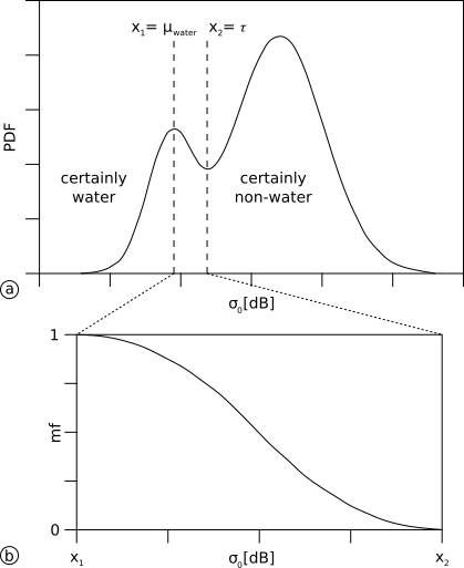
Figure 23: Fuzzy logic approach for discriminating water and non-water classes based on SAR backscatter values. (See text for details).
The diagram in Figure 23b depicts the membership function as the standard S-function, described in Pal et al. (1988). As high SAR backscatter values propagate to the threshold τ (low membership degree) and low SAR backscatter values propagate to the mean of the water class µwaterµ_{water}µwater (high membership degree), we negate the standard S-function (Figure 24).
In Figure 24, the positive S-function applies when assigning low pixel values with a low degree of membership and high pixel values with a high degree of membership. The negative S-function applies vice versa. Any SAR backscatter value that is less than or equal to µwaterµ_{water}µwater is assigned a high degree of membership, thus a fuzzy value of 1. Any SAR backscatter value that is greater than or equal to τ is assigned a low degree of membership, thus a fuzzy value of 0
Slope values equal to 0 have a high degree of membership, thus a fuzzy value of 1. Any slope that is greater than or equal to an empirically determined value of 18° has a low degree of membership, thus a fuzzy value of 0. For the slope, we also apply the negative S-function.
Considering the size of an area detected as water, we define a minimal, empirically determined mapping unit range of [10, 500], i.e. any water area with a size less than or equal to 10 pixels has a low degree of membership, thus a fuzzy value of 0. Any water area with a size greater than or equal to 500 has a high degree of membership, thus a fuzzy value of 1. For the minimal mapping unit, we apply the positive S-function.
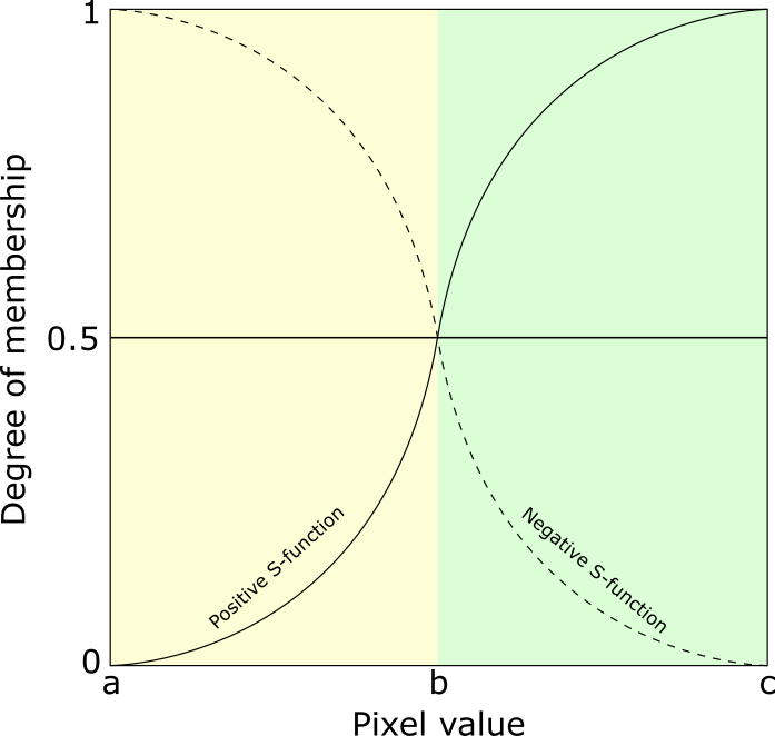
Figure 24: Standard S-function modified from Pal-Rosenfeld (1988). (See text for details).
The result of the fuzzy logic approach are three fuzzy layers in the range [0, 1]. For performance reasons, the float values were rescaled to the range [0, 100]. The resulting fuzzy layer is the mean of all three individual fuzzy layers.
A region-growing algorithm is applied as post-processing step, given the fuzzy layer and the initial water detection as inputs.
Water pixels with a fuzzy value of ≥ 0.6 are treated as correct water classifications. Water pixels with a fuzzy value of ≥ 0.45 and < 0.6 are treated as potential water pixels that are subject to region-growing.
Water pixels with a high fuzzy value of ≥ 0.7 are treated as seed pixels. Any potential water pixel, i.e. with a fuzzy value of ≥ 0.45 and < 0.6, that is also directly adjacent to a seed pixel is then remapped as a certain water pixel. As the original fuzzy value of that pixel was below the critical certainty mark of 0.6, we also remap the fuzzy value to the lowest uncertainty corresponding to the water class, i.e. 0.6.
As a final step, we further modify water detections based on the size of the region in which they are located. A region detected as water must have a minimum size of 30 pixels. Otherwise, that region is treated as a misclassification and remapped as land. The converse is also true, such that a region detected as land must have a minimal size of 10 pixels. Otherwise, the region is treated as a misclassification and remapped as water.
Any original water region that is remapped is assigned a fuzzy value representing land with a low classification accuracy, i.e. 0.45. Any original land region that is remapped as water is assigned a fuzzy value indicating water with a low classification accuracy, i.e. 0.6.
¶ Estimation of uncertainty for flood mapping algorithm 3 (TUW)
As mentioned in Section Masking of Sentinel-1 radar shadows, Algorithm 3 Bauer-Marschallinger et al, (2021) yields posterior probabilities of a backscatter measurement for belonging to either the flood or non-flood class. Based on the Bayes decision rule the higher posterior probability defines the class allocation. Additionally, the conditional error P(error│σ0)P(error│σ^0)P(error│σ0) can be defined by the lower posterior probability.

The conditional error as measure for the uncertainty allows directly to quantify the (non-) confidence of the provided decision. Since per definition the posterior probabilities sum up to 1, a higher posterior probability for one class results in a lower posterior probability for the other class. Consequently, the uncertainty is defined between 0.0 and 0.5. An uncertainty close to zero implies a very confident decision, since the probabilities for both classes (flood and non-flood) support a clear decision. The opposite condition would be an uncertainty of close to 0.5, which implies that the probabilities of the input Sentinel-1 value belonging to the two classes is nearly identical.
For all pixels of the incoming Sentinel-1 image, the conditional errors (P(error│σ0)P(error│σ^0)P(error│σ0)) are forwarded to the ensemble algorithm, representing the uncertainties of Algorithm 3’s flood mapping, per individual pixel.
In case of high conditional errors (i.e. close to 0.5), no certain decision can be made. In order to exclude such poorly based decisions (with low reliability), a dedicated uncertainty mask is already applied in Algorithm 3 (see Section 4.1.4 for more details).
¶ Output layer “Advisory flags”
Various meteorological factors may hamper or even prevent the detection of flooded areas. As discussed by Matgen et al. (2019) strong winds, rainfall, as well as the presence of wet snow, frost and dry soils are of particular concern. These factors are all important because they reduce the contrast between backscatter from open water surfaces and backscatter from the surrounding areas, thereby reducing the separability of flooded areas and surrounding land. While wind, frozen water surface and rainfall might reduce the backscatter contrast by increasing backscatter over water due to wind- and rainfall-induced roughening of the water surface, wet snow, frost and dry soils reduce the contrast by decreasing backscatter over the surrounding areas.
Unfortunately, all these factors are difficult to capture because of their extremely dynamic nature and high spatial heterogeneity. Therefore, wind, rainfall, temperature, and snow data coming from sparsely distributed meteorological stations and/or numerical weather prediction with its much coarser resolution are hardly suited to capture the exact situation at the time of the S-1 acquisition and are not ideal for providing the required advisory flags. It should be noted that optical remote sensing satellites such as MODIS or Sentinel-3 would provide sufficient spatial details, but neither do optical data depict the environmental conditions as seen by Sentinel-1, nor do they provide timely observations at all times due to cloud cover and poor lightning conditions. Therefore, in the scope of the GFM service, the only robust and applicable source for the environmental advisory flags is microwave remote sensing data. Our approach builds on using the S-1 NRT data and Sentinel temporal parameters (see section 3.1.2) that were derived from time series within the Sentinel-1 data cube archive.
The GFM product output layer “Advisory flags” aims for raising awareness that meteorological processes comprising wind or frozen conditions might impair the water body detection. As the here defined Advisory Flags can only be retrieved at a coarser resolution, we do not forward the information of the flags to the masking or to the Exclusion Mask. As coming in the form of the additional layer, it should guide the users when interpreting the product, allowing additional insight on its local reliability at the time of Sentinel-1 acquisition. The Advisory Flags indicate locations where the SAR data might be disturbed by such processes during the acquisition, but leaves the flood and water extent layers unmasked. In summary, pixels marked by the Advisory Flag are not excluded by the Exclusion Mask, but users are advised caution when using the observed water and flood extents over flagged areas. As outlined in the following section, the Advisory Flag layer consists of 2 separate flags, defining 4 potential flag values:

Figure 25 shows an example of the output layer “Advisory flags” for a Sentinel-1 scene over Greece from 2020-08-10 at 16:32 (from orbit A175), a point in time when windy conditions where prevalent. In Figure 25, the Advisory flags are overlaid on the backscatter image with transparent colours, with red for Low Regional Backscatter (Snow, Ice, or Dryness), green for Rough Water Surface (Wind), and blue for both.
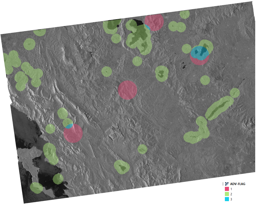
Figure 25: Example of the GFM product output layer “Advisory flags” for a Sentinel-1 scene over Greece from 2020-08-10 at 16:32 (from orbit A175), a point in time when windy conditions where prevalent. (See text for details).
¶ Algorithm for generating the Advisory flags
For the Advisory Flag layer production, we need to combine the near real-time input data flow, as well as read out the corresponding statistical parameters and auxiliary layers. After processing the flood extent for the incoming Sentinel-1 scene, the involved Equi7Grid-tiles are identified and the collocated parameters and auxiliary layers are read from the database. Figure 26 illustrates the data flow and how the flag values are set logically.
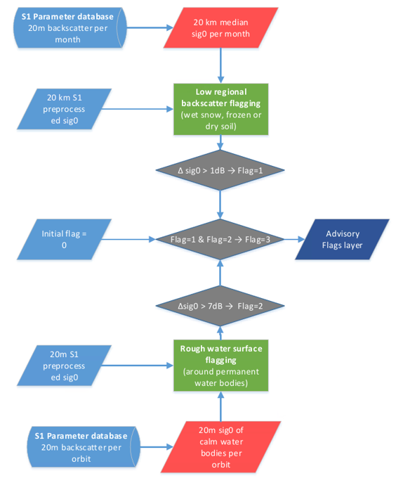
Figure 26: Advisory Flag workflow combining the low regional backscatter flag (Flag 1) and the rough water surface flag (Flag 2). The final Advisory Flags layer includes four values, 0 if no dynamic influence is present, 1 for Flag 1, 2 for Flag 2, and 3 if both flags are true.
¶ Low Regional Backscatter Flag
During the snow accumulation period, dry snow and ice-packs are almost transparent to microwaves. As a result, the SAR signal penetrates the snow / ice-pack up to several meters and the main contribution to the backscattering is from the snow–ground interface Rott et al. (1987). During the melting period, however, the increase of the amount of free liquid water inside the snow and ice bodies causes high dielectric losses, thereby increasing the absorption coefficient, featuring very low backscatter. In addition, the occurrence of meltwater puddles might change the backscattering behaviour of the surface, leading to components with specular microwave reflection, further decreasing the received amplitude at the sensor. Such patches of very low backscatter from those combined effects act easily as water-look-alikes and are source of false alarms.
Low backscatter over large regions characterizes all the above-described effects. Thus, to derive an Advisory Flag 1 called “Low Regional Backscatter”, we resample the Sentinel-1 acquisitions to 20 km resolution and compare the regional backscatter to the regional monthly grouped median value (see section 3.1.2) which represents seasonal backscatter signature of the corresponding region. Prior to resampling, each acquisition as well as the median image is masked using the reference water mask (see section 4.3), radar shadow mask (see section 4.4.1.3) and build-up area mask (see section 3.2.5). The difference between regional backscatter and regional monthly grouped median backscatter reveals regionally low backscatter values that are likely to be caused by snow, frost or dry conditions while taking the seasonal variations due to e.g., annual changes in vegetation cover into account. On the condition, that this difference exceeds 1 dB, the low backscatter flag is set to value “1”:

These values are subsequently resampled to the 20m pixel sampling and a simple radial buffer of 14 km radius is applied to the identified pixels with regionally low backscatter.
Known limitation of the used approach is the low number of flagged data in areas, where frozen or dry conditions are typical for full months (e.g., permanently frozen soil during winter months in northern regions).
¶ Rough Water Surface Flag
Wind, strong rainfall or frozen water surface over flood surfaces can lead to missed alarms, as they undermine the initial assumption of low backscatter due to specular reflection on smooth water surfaces. As a response to wind stress, short waves on the order of centimetres to decimetres are formed at the water surface causing an enhanced backscatter signal that occurs due to a constructive interference that reinforces the backscatter signal. This effect is called Bragg resonance effect and is dependent on wind speed and direction as well as on the radar wavelength. For C-Band, the minimum threshold wind speed that can cause this effect and thus enhance the backscatter from water surface is estimated to be 3.3 m/s. Similarly, strong rainfall events roughen the water surface and thus lead to the enhanced backscatter. In case of the frozen lake surface, the enhanced backscatter values are caused by the scattering from water/ice transitions. For the detection of these effects, we make use of the backscatter signature of permanent water bodies inferred from time series within the Sentinel-1 data cube archive.
We examine the NRT 20m Sentinel-1 backscatter data over the areas identified by the reference water mask (see section 4.3) and additional criteria based on backscatter. Concretely, for the pixel to be identified as water and used for the rough water surface flag decision, it needs to be identified as permanent or seasonal water body by the reference water mask of the given month and it has to have backscatter value below –10 dB and reference backscatter value (represented by the 5th percentile of Sentinel-1 sig0 backscatter) below –20 dB. The criteria based on backscatter are needed, as the water bodies shape might deviate from the seasonally defined reference water mask. For this reason, masking of very high backscatter values helps to avoid the situation, that the rough water surface mask would be issued due to the change of the water body shape instead of due to the roughening of its surface.
Over the identified water pixels, we examine, whether the backscatter deviates from a calm water signature. In the case of a roughened water surface, it is most likely to observe increased backscatter that is indicative of strong winds, rainfall, or frozen water surface, which in turn are likely to increase the backscatter from the nearby water surfaces over the flooded areas too.
For the calm water signature, we chose the 5th percentile of Sentinel-1 sig0 backscatter (see section 3.1.2) as baseline. An analysis of backscatter images at windy conditions led to the selection of 7dB difference as a threshold to distinguish rough from non-rough water surfaces, with respect to the local calm water signature. On the condition that this limit is exceeded over water surface, we set, on the 20m pixel scale, the rough water surface flag to value “2”:

As a final step, all pixels identified as roughened permanent water bodies are spatially filtered by using morphological operations. On the assumption that wind, rainfall or frozen water surface induced patterns are highly correlated within the neighbouring area, a simple L2/radial buffer of 5km radius is applied to the identified rough-water-surface-pixels, effectively enlarging the identified area. All pixels within the buffered area are labelled with the Advisory Flag 2 called “Rough Water Surface”. This should also reflect the initial expectation that the majority of floods appear in the vicinity of rivers and permanent or seasonal water bodies, and the wind flag is needed by users in those areas.
It should be noted that this realisation of the wind flag constitutes the initial version here in GFM. We foresee tweaking and optimisation (in respect to the 7dB threshold and the 5km radius) towards the alert accuracy, once more experience within the operational service is gained.
Finally, the 20m pixel array for the Advisory Flag is obtained from the combination of both intermediate flag outputs. All pixel locations that have values in the incoming Sentinel-1 image are initiated with value 0, and are updated with the following operation:

Effectively, all pixels with no flag set get the value 0, and all pixels where both flags are set get the value 3.
Known limitation of the used approach are flags that are issued due to the land cover change (e.g. water body changed its shape when compared to the reference water mask and the enhanced backscatter caused by this change is misinterpreted as roughened water surface). Generally, the quality of this flag is strongly dependent on the quality and topicality of the reference water mask.
¶ Output layer “S-1 metadata”
The GFM product output layer “S-1 metadata” consists of all available metadata attributes provided with each Sentinel-1 GRD data product used in the generation of the global flood monitoring product. Metadata of each Sentinel-1 GRD scene is encompassed in the distributed Sentinel “Standard Archive Format for Europe (SAFE)” format included in the “manifest.safe” file. The manifest file is an XML file containing the mandatory product metadata. Attributes contained in the manifest file are classified into four categories: summary, product, platform, and instrument. Platform and instrument related attributes are considered as static for the different Sentinel-1 satellites. A total number of 29 attributes are contained in the manifest file such as information about the absolute orbit number, pass direction, polarisation, sensing start and end date and the product timeliness category. An abstract of the included attributes is given in hereafter as an example.
Table 8: Example of metadata fields available in the corresponding layer.
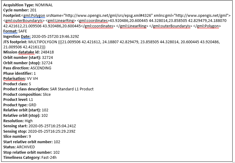
¶ Output layer “S-1 footprint”
The footprint of a Sentinel-1 GRD scene as provided in each data product is included in the before discussed manifest file. The footprint is represented as human readable Java Topology Suite (JTS) object named “JTS footprint”. The JTS footprint is converted into Well-known Text (WKT) and Well-known Binary (WKB) in the process of parsing and ingesting the acquired manifest files into the operated metadata database. WKT and WKB are originally defined by the Open Geospatial Consortium (OGC) to describe simple features. On-the-fly conversion to GeoJson is provided to aggregate the requested footprint features into the corresponding layer request by the user.
¶ Output layer “S-1 schedule”
Sentinel-1 observations follow a strict acquisition planning often referred to as acquisition segments. Information on the planned future acquisition is provided by ESA in form of Keyhole Markup Language (KML) files. A single file usually covers an acquisition period of about 12 days, with the start and stop time of the future planned acquisitions already given in the file name. KML files are publish by ESA on a regular base, well before activation, with potential last-minute changes due to requests from the Copernicus Emergency Management Service. Information provided by the KML files are organized based on the planned data takes. Parameters listed in following table are included in the KML. KML files are regularly checked, downloaded and ingested into the described metadata database for further analysis. All parameters are exposed in the layer to extract the requested schedule information indicating the next planned Sentinel-1 GRD acquisition for a given location.
Table 9: Information provided with the next planned Sentinel-1 GRD acquisition.
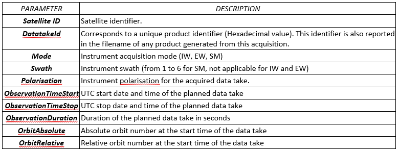
¶ Output layer “Affected population”
The information about the affected population is extracted from the Global Human Settlement Layer (GHSL), in particular the GHS-POP dataset. This data contains a raster representation of the population’s distribution and density as the number of people living within each grid cell. The information is available at various spatial resolutions and for different epochs. For the GFM service, we will consider the dataset at 100m resolution (highest possible resolution) and for the latest available time-step, 2020.
The dataset was re-projected to the same grid system as the flood map itself, which is the Equi7Grid with a 20m pixel-spacing and a 300km gridding (T3 level). Furthermore, the data was resampled from 100m to 20m resolution. The resampling was performed based on a nearest neighbour resampling and dividing input pixels by number of 20m pixels which fit into one 100m pixel (25).
The updated dataset replaces the former GHSL population dataset at 250m resolution with the reference year 2015 which was available at the start of operations and was used during production from October 2021 – March 2023.

¶ Output layer “Affected land cover”
Land cover information is extracted from the Copernicus Land Monitoring Service making use of the Global Land Cover dataset which is available at a global level with a resolution of 100m. The Copernicus Global Land Cover3 includes 23 classes and provides annual updates. The dataset was reprojected to the same grid system as the flood map itself, which is the Equi7Grid with a 20m pixel-spacing and a 300km gridding (T3 level). The data was then resampled from 100m to 20m resolution.
This information provides a first assessment of affected land cover or land use types, e.g. how much agricultural area is affected by the flood within the flood extent area or the area of interest.
Didn't find what you were looking for? Send us a message through the contact forms:
EFAS: https://european-flood.emergency.copernicus.eu/en/form/feedback [Flood Monitoring]
GloFAS: https://global-flood.emergency.copernicus.eu/contact-us/ [Satellite-based Global Flood Monitoring]