The TUW flood mapping algorithm, which was originally described by Bauer-Marschallinger et al. (2022), parameterizes a large fraction of the Sentinel-1 SAR backscatter signal history for each image pixel, which is stored within an extensive spatio-temporal datacube (or time-series) of SAR images that have been geocoded, gridded and stored as analysis ready data. As described in Section 2.1 of this report, the datacube contains the complete historical archive of Sentinel-1 SAR IW GRDH products acquired in VV (vertical transmit and vertical receive) polarisation, which are preprocessed, co-registered and time-stacked over the Equi7Grid global spatial reference system. The Sentinel-1 SAR image data are stored as backscatter coefficient values (σ0) in decibels, which have been resampled to a spatial resolution of 20 metres (from an original resolution of 10 metres), mainly for the purposes of noise reduction, as well as for optimal data storage and processing requirements.
The Sentinel-1 SAR image datacube serves as the source for two important datasets that are used by the TUW flood mapping algorithm, as described below: (a) the projected local incidence angle (PLIA) values, which describe the SAR observation geometry for each pixel; (b) the harmonic parameters, which describe the backscatter’s seasonality for each pixel.
The TUW flood mapping algorithm takes advantage of Sentinel-1 orbit repetition and a priori generated probability parameters for flood and non-flood conditions. A globally applicable flood signature is obtained from manually collected wind- and frost-free images, and provides expected backscatter Sentinel-1 values over water, depending on incidence angle. Through harmonic analysis of each pixel’s full time-series, a local seasonal non-flood signature is derived, comprising the expected backscatter values for each day-of-year over land pixels. From these predefined probability distributions, all incoming Sentinel-1 images are classified in near real-time by simple Bayes inference, also providing the uncertainty values that are ingested in the GFM likelihood layer.
The TUW flood mapping algorithm requires the following three main inputs datasets:
- the latest Sentinel-1 SAR image scene to be processed
- Sentinel-1 projected local incidence angle data (used to derive the Flood backscatter signature)
- Sentinel-1 harmonic parameters (used to derive the Non-flood backscatter signature)
In the following sub-sections, details are presented on the main datasets and analysis methods used by the TUW flood mapping algorithm, namely:
- Computation of Sentinel-1 projected local incidence angle data
- Computation of Sentinel-1 harmonic parameters
- Estimation of backscatter distribution functions for water and land surfaces
- Bayesian flood mapping and uncertainty estimation
- Low sensitivity masking
- Morphological post-processing
¶ 3.3.1 Computation of Sentinel-1 projected local incidence angle data
Under the conditions that water bodies are open, calm, and non-frozen, the Sentinel-1 SAR backscatter signal can be assumed to be of universal character, and primarily dependent on the (local) incidence angle of the incoming Sentinel-1 radar wave.
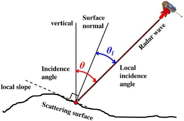
Given a point target on a scattering surface, characterized by a certain local slope, the local incidence angle (θl) is the angle between the incoming radar wave direction and the normal direction to the scattering surface. As can be seen in Figure 12, the local incidence angle (θl) differs from the incidence angle (θ), which is the angle between the incoming wave direction and the vertical direction to the ellipsoid. The projected local incidence angle (PLIA) is simply the local incidence angle projected into the range (i.e. across-track) plane. The PLIA provides essential information about the observation geometry of the satellite, and varies across different orbits.
The PLIA values are available as a by-product of the terrain correction step of the SAR preprocessing chain. Because of the self-repeating orbit geometries of the Sentinel-1 mission, almost identical observation angles are established at each overpass. Globally, the Sentinel-1 mission has 175 (repeating) relative orbits, with locally up to 9 orbits. Consequently, when working with Sentinel-1 data separately per relative orbit (r), a pixel’s PLIA value (θr) is assumed to be constant.
We capitalise on this, and use as input to the TUW flood mapping algorithm a set of constant θr values, which are computed a priori and per-orbit as average θ of the Sentinel-1A and 1B observations for the year 2020. As is described in Section 3.3.3 below, these mean PLIA values of the corresponding orbit are used together with the backscatter (σ0) images and the parameters of the harmonic model, as input for the TUW flood mapping algorithm.
¶ 3.3.2 Computation of Sentinel-1 harmonic parameters
The radar signal interacts with the Earth’s surface in many different ways. It can be absorbed, scattered, and reflected according to the surface states and characteristics of the sensor. The surface state (e.g. soil moisture content, vegetation, roughness) varies over time, leading to variation of backscatter time-series. Based on different periods of variation, time-series of backscatter can be decomposed into trend, seasonality and short-term random variation.
The TUW flood mapping algorithm utilizes a harmonic model to simulate the backscatter seasonal variation and to estimate normal, non-flooded conditions (see Section 3.3.3 below). This section describes the preparation performed to define the harmonic model on a global scale.
Following the approach of Bauer-Marschallinger et al. (2022), the TUW algorithm uses a harmonic model to compute the most probable radar backscatter (σ0) at time tday (i.e. day of the year), based on the harmonic parameters (𝐶𝑖, 𝑆𝑖, 𝝈̅̅𝟎̅ )The terms and definitions used to compute the harmonic parameters (i.e. the harmonic coefficients and the average backscatter) are described in Table 15.
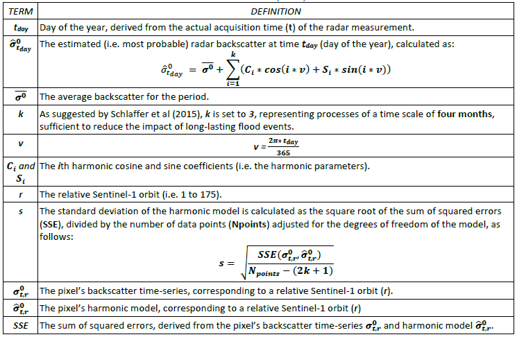
Table 15: Terms and definitions used to derive the parameters of the harmonic model describing the backscatter’s seasonality for Non-flood conditions. For details, see Bauer-Marschallinger et al. (2022) and Schlaffer et al (2015).
Figure 13 (panels a - d) show examples from the local non-flood distribution dataset for four selected days of the year, i.e. the expected backscatter for relative orbit D080 resulting from the harmonic analysis defined in row 2 of Table 15. Figure 13 (panels e - f) show, for two relative Sentinel-1 orbits (descending D080, and ascending A175), example temporal plots of the expected local distribution over observed backscatter (in green), and the water distribution for the local incidence angle (in red), which is static over time, with two low spikes corresponding to flood events.
Note that for Version 3.x of the GFM product, the harmonic parameters were updated, to improve accuracy over agriculture, for example. After evaluating impacts for different periods, the 3-year baseline period of 2019-2021 was selected as an optimal dataset, providing a best parameterization of the TUW algorithm in terms of data availability, orbit stability, and robust performance.
The harmonic parameters are derived from a least-squares estimation based on the backscatter values and corresponding observation times of input Sentinel-1 time-series. It should be noted that the derivation of the harmonic parameters within the GFM product differs from the method of Schlaffer et al (2015), as the backscatter values are used directly, instead of 10-day composites.
Backscatter coefficients are highly dependent on acquisition geometry. While a normalization approach could be utilized when sufficient incidence angle samples per pixel are present (as with ENVISAT ASAR), this is not feasible with Sentinel-1. Hence, parameter estimation is performed for each unique acquisition geometry, corresponding to a relative Sentinel-1 orbit. A unique set of harmonic parameters is required per orbit per Equi7grid tile. To model the estimated backscatter for any given day (t) and relative orbit (r), seven harmonic parameters are computed (for k = 3).
In order to measure how many samples support the estimation and to exclude ill-fitted harmonic parameters, the number of valid observations (NOBS) for each pixel is written as an additional layer. The standard deviation of the harmonic model is also calculated (see Table 15), based on the sum of squared errors derived from the pixel’s backscatter time-series and its harmonic model.
¶ 3.3.3 Estimation of backscatter distribution functions for water and land surfaces
The backscatter probability distribution functions for the Flood and Non-flood classes are derived based on dedicated statistical parameters generated from the Sentinel-1 multi-year data archive (i.e. the datacube), as described below. These distribution functions are subsequently used as input for the Bayesian flood mapping and uncertainty estimation, to compute the posterior probabilities for the Flood and Non-flood classes, as described in Section 3.3.4 below.
¶ 1. Flood backscatter probability density function:
Due to specular (or mirror-like) reflection of the radar pulses by water surfaces, the backscatter intensities received by the sensor are significantly lower compared with most other land cover types. A temporarily flooded surface is thus detectable by a significant decrease in its backscatter relative to the time-series. In order to ensure that the decrease is due to flooding, and no other effect, a detailed statistical knowledge of the backscatter behaviour over water surfaces is required.
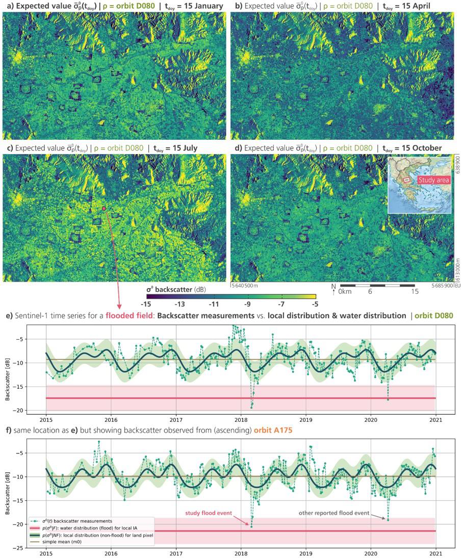
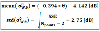
The proposed concept is to define the Flood backscatter probability density function (PDF), for any given (projected local) incidence angle (θ). It is assumed that the Flood backscatter PDF is a normal distribution, and can be parametrized by a mean and a standard deviation. Therefore, various observed backscatter values for water bodies and their respective incidence angles (further referred to as σ0W,θ) were collected from the Sentinel-1 datacube over oceans and inland waters. In Figure 14, the collected backscatter values (σ0W,θ) are plotted against incidence angle, which confirms the expected indirect dependence of water backscatter values and incidence angles.
For each specific incidence angle, the mean backscatter value was derived by linear regression. The slope of the regression of mean backscatter values (red line in top part of Figure 14) is 0.394. The slope of the regression of standard deviations (bottom part of Figure 14) is small (0.008), so “homoscedasticity” (i.e. same variance) is assumed. The total standard deviation is the square root of the sum of squares error (SSE), normalised with respect to the number of data points (Npoints).
Therefore, the Flood backscatter PDF (referred to as P(σ0 │ F)) is defined by its mean backscatter value and standard deviation, which are calculated per incidence angle as follows:
¶ 2. Non-flood backscatter probability density function:
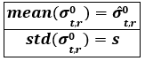
In order to model the normal, non-flooded conditions of each pixel in the Sentinel-1 SAR image datacube, we use the harmonic model described in Section 3.3.2 above. The harmonic model can be used to retrieve the expected backscatter value (𝝈̂0t,r) for any day of the year (tday) and specific relative Sentinel-1 orbit (r) (see Table 15). Therefore, the backscatter’s seasonality for each pixel in the datacube can be modelled by defining the harmonic parameters (Ci, Si, 𝛔̅̅𝟎̅), based on the pixel’s backscatter time-series (𝛔0r) (see Table 15). This harmonic model is used to define the Non-flood probability density function (PDF) for each pixel, which is assumed to be a normal distribution.
The mean backscatter value is set to the expected backscatter of the harmonic model (𝝈̂0t,r). As well as the harmonic parameters, the standard deviation (s) of the harmonic model is also computed (see Table 15), and is used as the standard deviation of the Non-flood PDF. Therefore, the Non-flood backscatter PDF (i.e. P(σ0 │ NF)), is defined by its mean backscatter value and standard deviation, which are calculated for each pixel in the Sentinel-1 SAR image datacube as follows (see Table 15):
Finally, a redundancy criterion is used to reduce the possibility of ill-fitting harmonic parameters (especially for locations with sparse data). This criterion is derived from the NOBS layer (see Section 3.3.2) which indicates the number of valid observations used to estimate the harmonic parameters.
Given the requisite [2k + 1] samples for a unique solution to the harmonic equation, the redundancy criterion is set as a multiple of this number. Since pixels not matching the redundancy criterion are excluded from the flood mapping, a balance must be found between number of excluded pixels and introduced noise. Based on initial tests, a redundancy value of 4 (e.g. 28 samples per pixel stack), can minimize noise, specifically at edges where sparse samples might be present.
¶ 3.3.4 Bayesian flood mapping and uncertainty estimation
Given the per-pixel knowledge of the relative orbit (r), day of year (tday), and incidence angle (θ), for each SAR image pixel one can define the parameters (mean and standard deviation) of the backscatter probability density functions (PDFs) for the Flood (F) and Non-flood (NF) classes (i.e. P(𝜎0 | F) and P(𝜎0 | NF), respectively). For each pixel in the new Sentinel-1 SAR image, the posterior (i.e. updated) probabilities of belonging to the Flood and Non-flood classes can then be computed, using Bayes theorem, based on the pixel’s backscatter value (𝜎0) and the Flood and Non-flood PDFs.
Recall that Bayes’ theorem is used to determine the posterior probability of a hypothesis (in our case Flood or Non-flood) being true, given new evidence (in our case backscatter value). The computation of the posterior probabilities is summarized in Table 16.
Table 16: Terms and definitions used to compute the posterior (i.e. updated) probabilities of pixels in a new Sentinel-1 SAR image belonging to the flood (F) and non-flood (NF) classes.
Note that the prior probabilities of the Flood and Non-flood classes (i.e. P(F) and P(NF)) shown in Table 16 represent the prior knowledge of the pixel belonging to a certain class. As no prior information is available, both probabilities are set to equal weight (i.e. 0.5). Furthermore, the marginal (or independent) probability of the backscatter value (i.e. P(𝜎0)) has the effect of scaling the values of the posterior probabilities to the range 0 to 1.
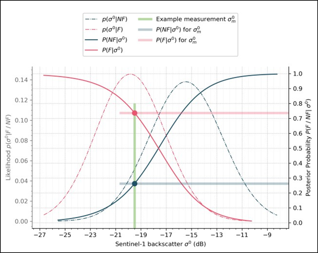
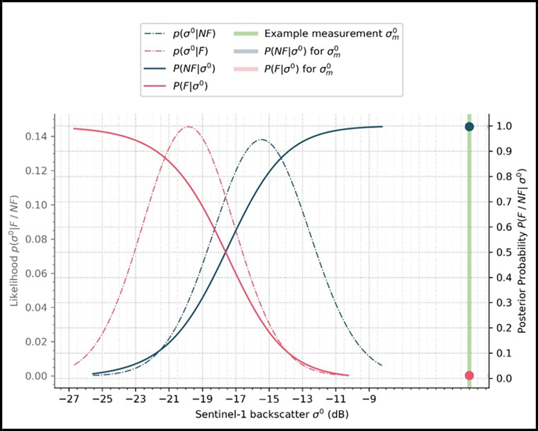
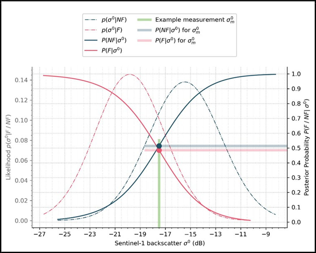
Bayes decision rule is then used to assign the pixel to the class (Flood or Non-flood) with the higher computed posterior probability. An example of the Bayesian flood mapping process for a single SAR image pixel, is illustrated in Figure 15, which includes both the probability distribution functions (i.e. P(𝜎0 | F) and P(𝜎0 | NF)) and the posterior probabilities (i.e. P(F | 𝜎0) and P(NF | 𝜎0)) for the Flood and Non-flood classes. As can be seen, the given backscatter value (-19.5dB) would be classified as flooded, since it has a higher computed posterior probability for the Flood class (P(F | 𝜎0)). Finally, a preliminary binary flood extent map is generated containing all pixels classified as flooded.
As can be seen in Table 16, the Bayesian flood mapping algorithm also provides the conditional error (i.e. P(error│σ0)), which directly quantifies the uncertainty of the classification. It is the lower posterior probability of the two classes (i.e. of the Non-flood class), and consequently its values are defined between 0.0 and 0.5, which are interpreted as follows:
|
|
|
¶ 3.3.5 Low sensitivity masking
To improve the reliability of the preliminary flood extent map generated automatically in near real-time by the TUW algorithm, a set of routines is applied to exclude those “low sensitivity” locations where the Bayes flood mapping does not allow a robust decision between flood and non-flood conditions. Therefore, four masks are generated that exclude pixels with (1) exceeding incidence angles, (2) conflicting backscatter distributions, (3) outlier values in backscatter distributions, and (4) high uncertainties of Bayesian flood mapping. Figure 16 shows an example of the four low sensitivity masks. The generation of the masks is summarized in Table 17, and described below.
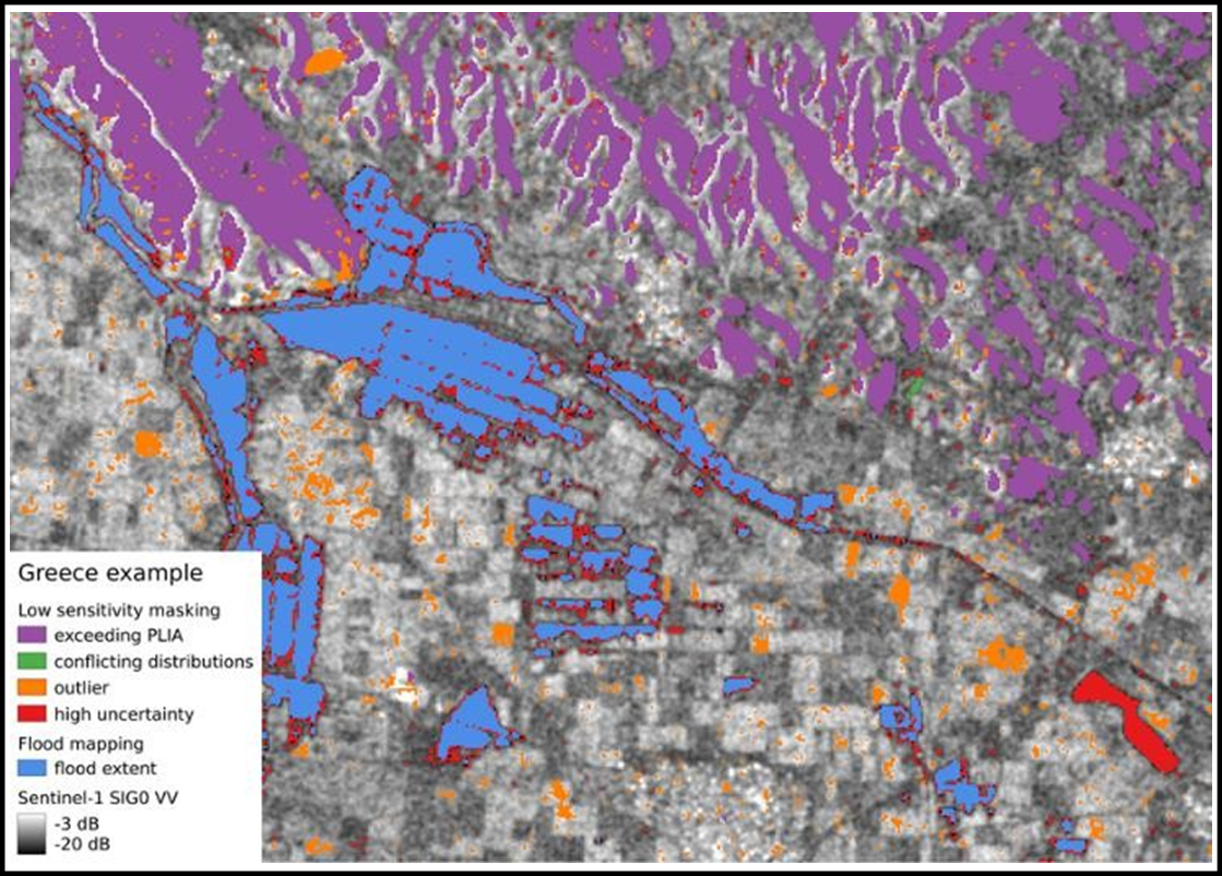
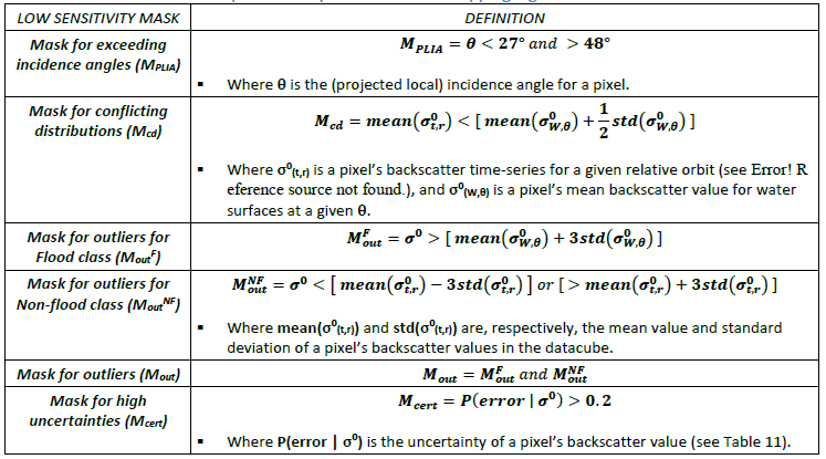
Table 17: Terms and definitions used for the low sensitivity masking of the preliminary flood extent map produced by the TUW flood mapping algorithm.
¶ 1. Mask for exceeding incidence angles:
Flat areas are observed by Sentinel-1’s IW mode at (projected local) incidence angles within the range 29° - 46°. By definition, this range includes (flat) water surfaces, and therefore the collection of water backscatter samples (described in Section 3.1.3.4) was limited to this range. In order to extend the flood mapping to gentle slopes, the range of incidence angles was relaxed to 27° to 48°, by applying a mask of exceeding incidence angles (see Table 17).
¶ 2. Mask for conflicting distributions:
The TUW flood mapping algorithm detects if a pixel that is normally non-flooded is temporarily flooded, implying that the pixel normally has a higher backscatter than a respective water surface. In other words, the Non-flood probability distribution function (PDF) must be higher overall than the Flood PDF. Typical locations where this condition is NOT fulfilled are permanent water, asphalt surfaces, salt flats, and very dry sand or bedrock areas. In addition to these “all-season” low backscatter conditions (permanent water, water look-alikes, etc.), a pixel’s backscatter may be low only for some seasons of the year, for example due to the rainy season, snow melting, etc. In order to exclude such areas showing conflicting distributions, a pixel is masked if the mean of the Non-flood PDF is lower than that of the Flood PDF plus half the standard deviation of the Water PDF (see Table 17). Figure 17 shows an example of a pixel that is masked due to conflicting distributions.
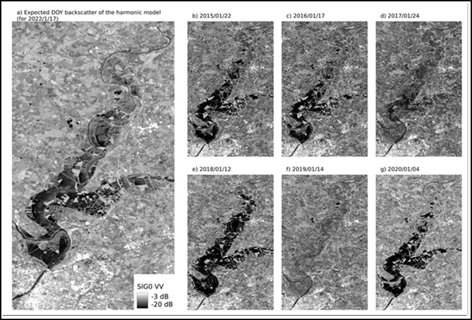
The consideration of such seasonal effects is an important feature of the harmonic model approach used by TUW algorithm (see Section 3.3.2). If the input observations for the harmonic model regularly show low backscatter for a certain season, the corresponding expected backscatter for a given day of the year should represent this. This is illustrated in Figure 18 for an area (near the city of Angers, France), where the expected backscatter for a given day of the year in 2022 shows a large area of low backscatter, which may be related to seasonal inundation. As can be seen in Figure 18, a similar pattern of inundations is observed also for other recent years. In this case, the harmonic model was trained within the current version (v3.x) of the GFM product, using data from 2019-2021, and appears to reflect the local dynamics in that perspective.
¶ 3. Mask for outliers:
The statistical model used by the TUW flood mapping algorithm is trained to provide robust decisions for normal flood conditions. Therefore, if the input backscatter value (σ0) is NOT represented by the Flood or Non-flood PDFs, the Bayes decision will not be reliable. In order to mask extreme values, only high outliers of the Flood PDF are considered, as it is assumed that low outliers of the Flood PDF can still be classified as flooded. The rule used for masking outliers is defined in Table 17. Figure 19 shows an example of such a situation with an outlier.
¶ 4. Mask for high uncertainties:
The conditional error produced by the Bayesian flood mapping (see Table 16) provides a measure of the confidence in the decision between Flood and Non-flood, and is used to limit the classification to certain decisions. Masking for high uncertainties is done by excluding pixels with P(error | σ0) > 0.2 (see Table 17). Figure 20 shows an example of the masking of an uncertain decision. As can be seen, the backscatter value is almost equally likely to be classified as Flood or Non-flood.
¶ 3.3.6 Final post-processing of the TUW flood map
Due to the coherent nature of the radar signal, a single Sentinel-1 image is affected by multiplicative noise (speckle). This random signal variation can lead to a noise-like pattern of pixels with lower or higher backscatter compared to their surroundings. Lower backscatter might be confused with flooded conditions, while higher backscatter could prevent a correct flood classification. With GFM v4.0, to reduce the influence of speckle on the flood extent map, a minimum mapping unit (MMU) of 17 pixels is applied and holes smaller than 7 pixels are filled. The result of this step represents the final flood extent and estimated uncertainty of the TUW flood mapping algorithm.
¶ 3.3.7 Computation of Likelihood Values by the TUW flood mapping algorithm
The TUW flood mapping algorithm estimates the uncertainty of flood classification (P(error │ 𝜎0)) for each grid-cell, as the minimum of the two posterior probabilities of the flood and non-flood classes (P(F | 𝜎0) and P(NF | 𝜎0)) (see Table 16). In order to be used by the GFM Ensemble flood mapping algorithm (see Section 3.4), these uncertainty values are “flipped”, so that low uncertainty values propagating towards 0 (indicating high likelihood of non-flood) are remapped to high likelihood values propagating towards 100 (indicating high likelihood of flood), and vice versa.