The LIST flood mapping algorithm, which was originally described by Chini et al. (2017), is a change detection approach that requires the following three main input datasets:
- the most recent Sentinel-1 SAR image sceneto be processed (It0), i.e. new image.
- the previously recordedoverlapping Sentinel-1 SAR image scene (It0-1), i.e. reference image.
- the corresponding previous GFM outputlayer Observed Flood Extent, generated by the GFM ensemble flood mapping algorithm.
The LIST flood mapping algorithmconsists of four main steps, which are described below:
Change detection by computing the difference betweenthe reference and new images.
- parameterizing the target and background distribution functions using a hierarchical split- based approach (HSBA).
- mapping the target class by HSBA-based histogram thresholding and region growing.
- final post-processing of the flood map produced by the LIST algorithm.
¶ 3.1.1 Change detection by computing difference between the reference and new images
In order to compute the changes between the reference image (It0-1) and the new image (It0), a difference image (ID) is computed as the difference between the reference image and the new image, i.e. ID = It0-1 - It0, with flooded pixels in the difference image expected to be positive because of the reduction of backscatter values caused by flooding.
The LIST flood mapping algorithm aims at detecting and mapping all increases and decreases of floodwater extent with respect to the reference image. As it is a change detection approach, this enables the differentiation of floodwater from permanent water bodies, as well as the filtering out of classes having water-like backscatter values, such as shadows or smooth surfaces. Moreover, in order to reduce false alarms caused by different types of unrelated changes (e.g. vegetation growth), a reference image acquired close in time to the new image is used.Sentinel-1 is well suited for this latter requirement, due to its repeat cycle of 6 days. Finally, in order to reduce false alarms further, and to speed-up the analysis, the approach uses as optional input data the Exclusion Mask and the HAND (Height above Nearest Drainage) terrain map.
Each time a new image scene is ingested and pre-processed, the algorithm processes the pair of scenes consisting of the new image (It0) and previous overlapping image from the same orbit (It0-1). A new flood map (FMt0) is generated, updating the most recent ensemble flood map (FMt0-1).
As in all statistical change detection or water mapping algorithms applied to SAR imagery, the parameterization of the distributions of the change (i.e. flood) and water classes depends on how easily identifiable the respective classes are in the histogram of backscatter values in the SAR imagery. More explicitly, classes such as flooded or changed areas typically represent only a small percentage of the total image, and so may not be easily identifiable on the histogram.
In order to address such a limitation, the LIST flood mapping algorithm uses a hierarchical split- based approach (HSBA) to locate specific regions (or tiles) of the difference image (ID = It0-1 - It0), and the corresponding new image (It0), where:
- The tile histogram is clearly bimodal, with two distributions representing the respective target (i.e. flood or water) and background (i.e. non-flood or non-water) classes.
- The two distributions in the tile histogram are Gaussian, and present with a similar frequency.
The logarithmic transformation that is applied to the backscatter values of Sentinel-1 SAR Ground Range Detected (GRD) images has the effect of converting the multiplicative noise (speckle) of SAR imagery to additive noise (which can be more easily removed), and increasing the dynamic range of low-intensity pixel values. Furthermore, the pixel values in a log-transformed image can be assumed to have a Gaussian distribution.
The “log-ratio” is a standard technique for change detection of SAR images, based on a pixel-by-pixel comparison of two images acquired at different times. The advantage of the log-ratio operator is that it takes account of the multiplicative model of speckle, and is also less affected by radiometric errors, so that the statistical distribution of the final image depends only on the changes between the two images. The log-ratio image is computed as the difference between the log-transformed reference and new images (i.e. ID = It0-1 - It0), based on the quotient rule for logarithms, namely:
- log(x / y) = log(x) - log(y)
Briefly, the distribution functions for the target (i.e. change and water) and background (i.e. non-change and non-water) classes in the difference and new images (ID and It0) are parameterized, using HSBA. The target and background distributions are then used to map the target classes in ID and It0, by histogram thresholding and region growing. In the region growing, the posterior probabilities of the target classes are used for the purposes of comparison with a threshold value, for selecting seed pixels for region growing, and a tolerance criterion, for stopping the region growing.
¶ 3.1.2 Parameterizing the target and background distribution functions using HSBA
Considering a SAR image, with backscatter measurements y, it is assumedthat:
- two classes are present, where G1(y) and G2(y) are their distribution functions.
- both distributions can be approximated by Gaussian curves.
- the prior probabilities of the two classesare strongly imbalanced.
This last assumption is typical for SAR images covering large areas, where changes only affect a small part of the image. When this happens, the smaller class is dominated by the other class, and its distribution is practically indistinguishable in the global histogram, thereby causing the classification problem to be ill-posed, and the selection of the threshold highly uncertain (Gong et al., 2016; Aach et al., 1995). In order to cope with the problem of imbalanced populations, regions (or tiles) of the SAR image where the two classes are more balanced are identified using a hierarchical split-based approach (HSBA), which consists of the following two steps, which are described below:
- Hierarchical tiling using quadtree decomposition
- Selection of tiles that are statistically representative
¶ Hierarchical tiling using quadtree decomposition:
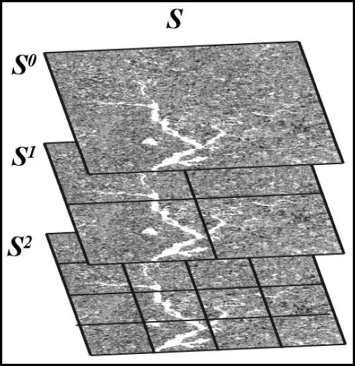
The first step in the HSBA is the hierarchical tiling of the SAR image using quadtree decomposition, which iteratively splits image regions into four quadrants, sub-quadrants, etc. Note that a quadtree is a hierarchical data structure that is used in image processing to partition recursively a two-dimensional image into four equally-sized quadrants or regions. Quadtrees are useful because of their ability to focus on the interesting subsets of the image.
Figure 4 illustrates the hierarchical tilingof a SAR image usinga three-level quadtreedecomposition. At each level of the quadtree, each quadrant or sub-quadrant corresponds with a specific node, representing a specific region (or tile) of the image, and has exactly four children, or no children at all. The latter is referred to as a leaf node. The first level of the quadtree (called the root node) represents the entire image region, while the last level of the quadtree (containing the leaf nodes) represents the smallest tiles (Laferte et al., 2000). For a quadtree with N levels, the set of nodes at the ith level of the quadtree (i.e. Si) contains 4i nodes, where i ∈ [0, N-1]. For example, the set of nodes at the last level (i.e. S2) of the quadtree shown in Figure 4 contains 42 = 16 nodes.
To summarize, for the hierarchical tiling of a SAR image (I) using an N-levelquadtree decomposition:
|
|
|
|
|
|
Thus, the resulting quadtree decomposition can be expressed as:
- 𝐒 = {𝐒𝟎, 𝐒𝟏, . . . , 𝐒𝐢 |⋃ 𝐈[𝐒𝐢] = 𝐈 = 𝐈[𝐒𝟎], 𝐰𝐡𝐞𝐫𝐞 𝐢∈ [𝟎, 𝐍 − 𝟏] 𝐚𝐧𝐝 𝐣∈ [𝟏, 𝟒𝐢]}
¶ Selection of tiles that are statistically representative:
For a SAR image (I), the histogram of any tile in the N-level quadtree (consisting of the set of nodes Sij, where i ∈ [0, N-1] and j ∈ [1, 4i], as described above) is expressed as h(I[Sij]).
An image tile I[Sij] is selected for estimating the parameters of the Gaussian distributions of the target and background classes (to be used for the histogram thresholding and region growing of the SAR image), according to the following three conditions:
|
Condition 1: |
|
|
Condition 2: |
|
|
Condition 3: |
|
Recall that in mathematics, a Gaussian function of a normally distributed random variable x, with mean μ and standard deviation σ, is of the form:
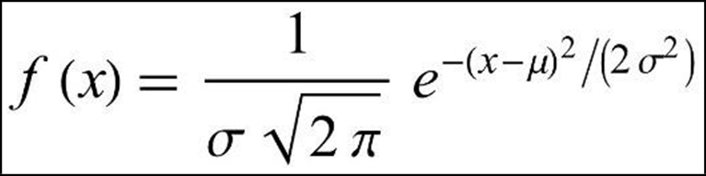
where 𝟏 / 𝝈 √𝟐 𝝅 is the function’s maximum value (amplitude or height), which occurs at x = μ.
For a SAR image (I), we hypothesize that the histogram of each tile, h(I[Si ]),is a sum of two Gaussian distributions (G1 and G2), i.e.:
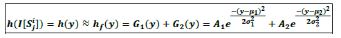
where the abbreviations are defined as follows:
| y : | The measurement (backscatter) |
| h(y) : | The tile histogram of image values. |
| hf(y) : | The distribution fitted to the tilehistogram. |
| A1, μ1, σ1 : | Amplitude (height), mean, standard deviation of the target distribution. |
| A2, μ2, σ2 : | Amplitude (height), mean, standard deviation of the background distribution. |
The parameters of the two Gaussian distributions that together composethe histogram of each tile in the SAR image, are estimated using the Levenberg-Marquardt algorithm.
The Levenberg-Marquardt algorithm is a standard technique for estimating the parameters of the distribution functions that best fit a set of empirical data. It solves the non-linear least squares problems by combining the steepest descent and inverse-Hessian function fitting methods (Marquardt et al., 1963). Non-linear least squares methods involve an iterative optimization of parameter values to reduce the sum of squares errors between a fitting function and histogram values. Iterations are done until three consecutive repetitions fail to change the chi-squared value by more than a specified tolerance, or until a maximum number of iterations has been reached.
When the Levenberg-Marquardt algorithm is applied, the initial guess of the parameters should be as close as possible to the actual values, otherwise the solution may not converge. The first-guess values are retrieved using Otsu's method (Otsu et al., 1979), an automatic image thresholding algorithm which in its simplest form returns a single intensity threshold that separate pixels into two classes, foreground and background.
Given the Otsu-derived threshold yot for the tile histogram h(y), the first-guess values of the amplitudes (A01, A02 ), means (μ01, μ02 ), and standard deviations (σ01 , σ02) of the two distributions G1(y) and G2(y), can be derived as follows:
| First-guess parameters for G1(y): | First-guess parameters for G2(y): |
|
|
|
|
|
|
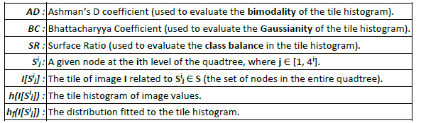
Once the distributions are fitted to all tile histograms in the SAR image, the statistical properties of each tile histogram are evaluated according to three conditions: only tiles with a bimodal histogram (Condition 1), and with two distributions that are Gaussian (Condition 2) and balanced (Condition 3), are selected for parameterizing the target and background distributions. The statistical properties of the tile histogram, and the indices used to evaluate them, are summarized in Table 8.
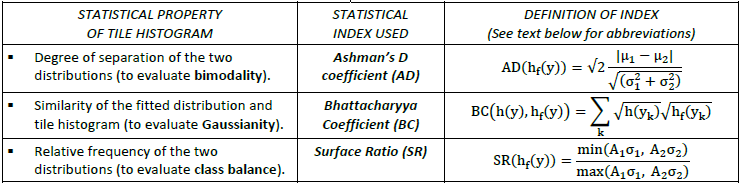
Table 8: The specific statistical properties, and corresponding statistical indices, used to select SAR image tiles that are suitable for parameterizing the target and background distributions.
where the abbreviations are defined as follows:
| y : | The measurement (backscatter) |
| h(y) : | The tile histogram of image values. |
| hf(y) : | The distribution fitted to the tilehistogram. |
| k : | The corresponding bin of the fitted and tile histograms. |
| A1, μ1, σ1 : | Amplitude (height), mean, standard deviation of the targetdistribution. |
| A2, μ2, σ2 : | Amplitude (height), mean, standard deviation of the background distribution. |
The three statistical indices which are listed in Table 8, and which are used to evaluate the bimodality (Condition 1), Gaussianity (Condition 2) and class balance (Condition 3) of the distributions of the tile histograms, are briefly described as follows:
|
STATISTICAL INDEX |
DESCRIPTION |
REFERENCE |
| Ashman’s D coefficient (AD): |
|
|
| Bhattacharyya Coefficient (BC): |
|
|
| Surface Ratio(SR): |
|
An overview of the procedure for selecting those tiles in the SAR image with a bimodal histogram (i.e. Condition 1), and two Gaussian and balanced distributions (i.e. Conditions 2 and 3), evaluated using the three statistical indices described above, is provided in Table 9 below.
In summary, for a given SAR image (I), the tiles of the entire N-Level quadtree are scanned from the set of nodes at level (i.e. S0) to the set of nodesat level N-1 (i.e.SN-1). Any node (and its associated image tile) that fulfils the following three conditions (C1, C2, and C3) is finally selected, and its “children” (i.e. tiles at subsequent levels in the quadtree) are not considered as candidate tiles:
- C1 (I[Sij]) = C2 (I[Sij ]) = C3 (I[Sij]) = 1 (see Table 9 below).
These processing steps result in a binary map, called a bimodal mask (BM), which includes regions in image I where the distinctive populations, G1 and G2, are present with a sufficient number of pixels, and where their distribution functions are clearly identifiable, and with more balanced prior probabilities. At this point, all tiles fulfilling the three conditions are selected, and thehistogram of all pixels enclosed by these tiles (i.e. where BM=1) must be clearly bimodal.
Finally, the histogram h(I[where BM=1]) is used to estimate the parameters of the Gaussian distributions of the target and background classes (i.e. GBM1(y) and GBM2(y)). To do so, the Levenberg-Marquardt algorithm is applied again, this time to fit two Gaussian curves on the histogram of pixel values included in all selected tiles.
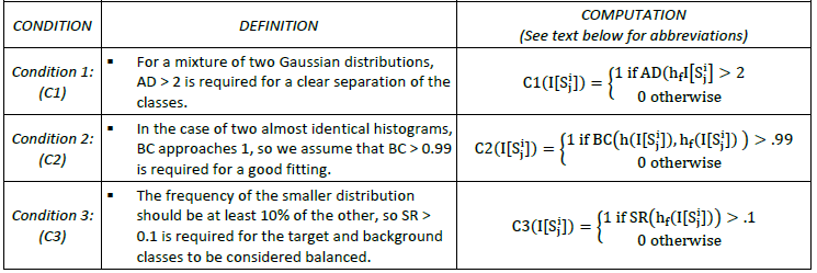
Table 9: Overview of the procedure for selecting statistically representative tiles, based on the evaluation of bimodality (Condition 1), Gaussianity (Condition 2), and class balance (Condition 3).
where the abbreviations are defined as follows:
¶ 3.1.3 Mapping target class by HSBA-based histogram thresholding and region growing
The LIST flood mapping algorithm first parameterizes the target (i.e. water and change) and background (i.e. non-water and non-change) distributions in the new and difference SAR images (It0 and ID), using HSBA. The four distributions are then used to apply a histogram thresholding and region growing, in order to map the target classes (water and change) in It0 and ID.
The LIST flood mapping algorithm must handle different flood events, lasting from a few days to weeks (e.g. monsoon events). Thus, the algorithm addresses two different possible cases:
- increased and recededfloodwater in the new SAR image.
- only receded floodwater in the new SAR image.
If neither of the cases is satisfied, meaning that the floodwater in the new SAR image (It0) has not changed relative to the previous SAR image (It0-1), the previous flood map (FMt0-1) is not updated.
The way the LIST flood mapping algorithm is implemented for both cases, is explained below.
¶ Case 1 - Increased and receded floodwater in the new SAR image:
In the first case, the hierarchical split-based approach (HSBA) described earlier is applied in parallel to the new and difference SAR images (It0 and ID), and the resulting bimodal mask is used to estimate the target and background distributions in It0 and ID. The estimated distributions are then used to apply a “two-input” region growing of both It0 and ID. A new flood map (FMt0) is created by adding the new floodwater in It0 to the previous flood map (FMt0-1). In addition, any floodwater in FMt0-1 that has receded in It0, is removed from FMt0.
The target and background distributions in It0 and ID are first estimated using HSBA, as follows:
|
|
|
|
|
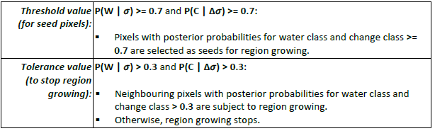
Region growing assumes that the pixels of the target classes (i.e. water and change) in the new and difference SAR images are clustered, not randomly spread out over the entire image. The region growing algorithm that is used to map the target class requires two parameters: a threshold value for selecting seed pixels, and a tolerance value for stopping the region growing. In the region growing, the threshold and tolerance values are used (as described below) for the purposes of comparison with the posterior probabilities computed for the target class, which are inferred from the fitted distributions of the target and background classes, via Bayes’ theorem (see Table 10).
| TERM | DESCRIPTION |
| A, B : | Event A (the hypothesis), event B (the evidence). |
| P(A ∣ B) : |
The posterior (updated) probability of event A, given event B, which is inferred as: P(A ∣ B) = P(B ∣ A) * P(A) / P(B) |
| P(B ∣ A) : | Conditional probability (or likelihood) of B, given A. |
| P(A) : | The prior (independent) probability of A. |
| P(B) : | The marginal (independent) probability of B. |
Table 10: Terms and definitions used to determine the posterior (or updated)probability of a hypothesis being true, given new evidence, using Bayes’ theorem.
How the target and background distributions are used to compute the posterior probabilities for the target classes in the new and difference SAR images, which are then compared with the threshold and tolerance values in region growing, is summarized in Table 11 and Table 12 below.
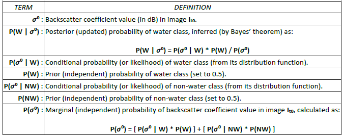
Table 11: Terms and definitions used to compute the posterior probabilities of the water class in the new SAR image (It0), for comparison with the threshold and tolerance values in region growing.
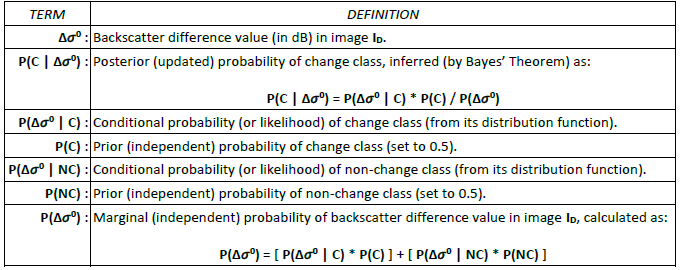
Table 12: Terms and definitions used to compute the posterior probabilities of the change class in the difference SAR image (ID), for comparison with the threshold and tolerance values in region growing.
The posterior probabilities for the target classes (water and change) in the new and difference SAR images are first used to select seed pixels for region growing, by a comparison with the threshold value. Selected seeds occurring in the height above nearest drainage (HAND) mask are removed, in order to avoid that false alarms (in areas not prone to flooding) could spread. Starting from the seed pixels, region growing is applied to neighbouring pixels with posterior probabilities within a specified range of tolerance values. The exact procedure is summarized as follows:
Any new floodwater detected by the application of the region growing procedure to the new and difference SAR images (It0 and ID), is added to the previous flood map (FMt0-1), producing a new flood map (FMt0). The algorithm must also remove from FMt0-1 any floodwater that may have receded in the new SAR image (It0).
To do this, the previously estimated water and non-water distributions are used to apply a “single-input” region growing of only the new SAR image (It0), in order to map the water in It0. Only pixels that are floodwater in the previous flood map (FMt0-1) and water in the new SAR image (It0) are mapped as floodwater in the new flood map (FMt0).
¶ Case 2 - Only receded floodwater in the new SAR image:
If the bimodal map resulting from applying HSBA in parallelto It0 and ID (described above) is empty, this means that any floodwater in the previous SAR image (It0-1) has either only receded or has not changed in the new SAR image (It0). To remove any receded floodwater in It0 from the previous flood map (FMt0-1), HSBA is re-applied, but only to the new image (It0), not in parallel to It0 and ID. The estimated water and non-water distributions are then used to apply a “single-input” region growing, in order to map the water in It0. Again, only pixels that are floodwater in the previous flood map (FMt0-1) and water in It0, are mapped as floodwater in the new flood map (FMt0).
¶ 3.1.4 Final post-processing of the LIST flood map
¶ Incidence angle-based processing and mask application:
The Observed Flood Extent output layer generated by the LIST flood mapping algorithm is processed using the GFM Exclusion Mask, the Height Above Nearest Drainage (HAND) mask, and the ocean pixels of the Copernicus DEM (Water Body Mask), to remove all pixels not part of flood-prone areas.
It should be noted that the LIST flood mapping algorithm is applied separately to strips that are a subset of the original input Sentinel-1 image, each strip having a narrower range of incidence angles. This reduces the impact of angle-dependent signal variations, which arise because backscatter can vary across an image, depending on the angle at which the radar signal hits the ground.
In general, backscatter decreases with increasing incidence angle. This dependency is observed for most land cover classes, but is most significant for smooth surface classes (e.g. water). For SAR wide-swath data, the backscatter distribution of a given class varies from near- to far-range. If the class of interest extends over the entire image, significant differences between incidence angles hamper the attribution of a unique backscatter distribution function.
Splitting the image into strips therefore improves the parameterization of the distribution functions of both the target (water and change) and background (non-water and non-change) classes in each strip. Each Sentinel-1 image is split into three strips, using incidence angle as a metric, as follows:
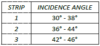
In order to avoid creating gaps in the flood map where flooding covers multiple strips, the borders between strips overlap slightly. This ensures a smooth flood map, even for large flood zones. In short, splitting the image with overlap improves the accuracy of the parametrization of the target and background distribution functions, by considering the effect of incidence angle on the radar signal. As an added benefit, processing the Sentinel-1 image in separate strips enables them to be analysed simultaneously, making processing much faster.
¶ Topography-informed object-based filtering:
The Observed Flood Extent output layer is further refined through a topography-informed, object-based classification and filtering approach. The purpose of this post-processing step is to preserve the most probable (“true”) flood extent while mitigating potential over-detection using HAND data.
First, the flood extent is segmented into discrete flood objects (F) based on D8 flow-direction connectivity. For each flood object, a two-pixel-wide buffer (B) is subsequently generated through two iterations of a 3x3 morphological dilation. Pixels within the buffer that overlap the water body mask are excluded from further analysis. The corresponding HAND values within both the flood objects and their buffers are then extracted for comparative evaluation.
This approach relies on the physical assumption that the HAND value distribution of a genuine flooded area should be shifted toward smaller values compared to that of its immediate surroundings, reflecting the gravitational tendency of water to accumulate within local topographic depressions. Thus, the statistical characteristics of the HAND value distributions within each flood object and its buffer are evaluated and classified according to five topography-based filters:
|
1 |
True filter: |
|
|
2 |
Bi-modality filter: |
|
|
3 |
Overlap filter: |
|
|
4 |
Mean difference filter: |
|
|
5 |
Mode filter: |
|
Flood objects that do not meet the criteria of any of the five filters are classified as Class 6 (Unclassified) and are conservatively retained as potentially true flood objects. In cases where multiple filters assign conflicting classes to a single object (e.g. “True” and “High-mode”), a hierarchical overwriting sequence is applied in the order 5 > 4 > 3 > 2 > 1, ensuring a consistent and physically meaningful classification outcome. This hierarchy reflects the relative confidence in identifying potential over-detections, whereby filters associated with stronger evidence of implausibility (e.g., a high-mode flood object) take precedence over those with weaker or more ambiguous conditions (e.g., overlapping distributions). For instance, if a flood object is simultaneously identified as both Class 1 and Class 4, it is finalized as Class 4 according to this rule.
Following the topography-informed filtering, flood objects classified as Classes 1, 2, and 6 are retained, representing plausible inundated areas. Conversely, flood objects classified as Classes 3, 4, and 5 are re-labelled as non-flood pixels, representing likely instances of over-detection.
¶ 3.1.5 Computation of Likelihood Values by the LIST flood mapping algorithm
The LIST flood mappingalgorithm estimates the likelihood of flood classification using the posterior probabilities (P(W | 𝜎0) and P(Δ𝜎0 | C)) computed for the water class in the new image and the change class in the difference image (see Table 11 and Table 12). For the two cases described in Section 3.1.3, the Likelihood Values are computed using two different methods, as described below.
For Case 1 (i.e. increased and receded floodwater in the new SAR image), both the new (It0) and difference (ID) SAR images are used to estimate the Likelihood Values.In this case, those pixels with high posterior probabilities for both water and change classes (i.e. (P(W | 𝜎0) and P(Δ𝜎0 | C)) are likely to be floodedpixels.
Therefore, a grid-cell’s probability of being flooded (P(F | 𝜎0)) is computed as the minimum value of the posterior probabilities for the water and change classes, as follows:
- P(F | 𝜎0) = minimum[ P(W | 𝜎0), P(Δ𝜎0 | C) ]
For Case 2 (i.e. only receded floodwater in the new SAR image), only the new SAR image (It0) is used to estimate the Likelihood Values. In this case, a grid-cell’s probability of being flooded (P(F | 𝜎0)) is computed as the posterior probability for the water class, as follows:
- P(F | 𝜎0) = P(W | 𝜎0)
It should be noted that, for Case 2, because the likelihood is only calculated from the backscatter value in the new image (It0), false high flood probability can be caused by permanent water and other water look-alike dark areas. Such false alarms in the binary flood map have been removed by comparing the map with the previous flood map, as described above. To reduce these false high probabilities in the current likelihood map, for non-flood pixels in the new flood map, the flood probability (P(F | 𝜎0)) is the minimum value between the posterior probability for water (P(W | 𝜎0) in the new SAR image and the probability of being flooded (P(F | 𝜎0)) in the previous likelihood map.
Finally, for both Cases 1 and 2, for grid-cells in the GFM Exclusion Mask, flood probability is set to 0.