The Global Flood Monitoring (GFM) product of CEMS provides a continuous monitoring of floods worldwide, by processing and analysing in near real-time all incoming Sentinel-1 SAR images acquired in Interferometric Wide Swath (IW) mode, and generating the ten output layers of flood-related information (see Table 1). In this Section, the key technical features underlying the generation of the ten GFM output layers of flood information, are described in detail.
¶ 4.1 GFM output layer: Observed Flood Extent
The GFM output layer Observed Flood Extent shows the flooded areas which are mapped in near real-time from Sentinel-1 satellite imagery, using three individual, state-of-the-art flood mapping algorithms (LIST, DLR, and TUW). Briefly, for each input Sentinel-1 SAR image scene, the three independent flood maps that are generated by the three individual flood mapping algorithms are combined into a single Observed Flood Extent output layer, using the GFM Ensemble flood mapping algorithm. Detailed technical descriptions of the LIST, DLR, TUW, and Ensemble flood mapping algorithms, which form the core of the GFM product, are provided in Section 3 of this PDD.
The results of the individual flood mapping algorithms are harmonized using the GFM Reference Water Mask and Exclusion Mask, respectively, to remove permanent (and seasonal) water bodies, and to exclude surface types where SAR-based water mapping is unreliable. The Observed Flood Extent and Likelihood Values are corrected by changing Flooded grid-cells included in the Reference Water Mask , to Unflooded. The Copernicus Water Body Mask is used to mask out ocean areas. The GFM Reference Water Mask and Exclusion Mask are described in Sections 4.3 and 4.4 below.
¶ 4.2 GFM output layer: Observed water extent
The GFM output layer Observed Water Extent identifies grid-cells classified as open and calm water based on Sentinel-1 SAR backscatter intensity, and is derived by combining (using a logical OR) the flood map generated by the GFM ensemble algorithm (see Section 3.4) with the seasonal and permanent water of the GFM Reference Water Mask (see Section 4.3 below). The values of the GFM output layer Observed Water Extent are defined in Table 19.
| VALUE | DESCRIPTION | USER INTERPRETATION |
|
0 |
No Water |
|
|
1 |
Water |
|
|
NaN |
No data available |
|
Table 19: Data values of the GFM output layer Observed Water Extent.
¶ 4.3 GFM output layer: Reference Water Mask
The GFM output layer Reference Water Mask outlines grid-cells that are classified as both permanent and seasonal water, using an ensemble water mapping algorithm (described below), and based on Sentinel-1 SAR median backscatter intensity over a certain time period, defined as follows:
- Permanent water extent is mapped based on each grid-cell’s median backscatter of all Sentinel-1 data over a reference period of five years.
- Seasonal water extent is based on each grid-cell’s median backscatter of all Sentinel-1 data for a given month over the same reference period.
Therefore, 12 monthly reference water masks are created, providing information on permanent and seasonal reference water extent.
The use of a permanent water mask is reliable in environments with stable hydrological conditions over the year. In regions with strong hydrological dynamics and spatio-temporal variations in observed water extent (e.g. areas affected by monsoons), the additional use of a seasonal reference water mask is desirable, as it also considers the seasonality of the observed water extent.
Unlike the GFM Ensemble flood mapping algorithm, the Ensemble water mapping algorithm uses only the LIST and DLR algorithms. The TUW algorithm is specifically designed to detect temporary flooded areas. It does not produce a water extent map, and is unsuited for the generic task of water mapping. The key elements of the Ensemble water mapping algorithm are summarized below:
|
|
|
|
Figure 26 shows an example (in Myanmar) of the GFM monthly reference water masks. Seasonal (i.e. monthly) variations of water bodies can be separated from permanent water bodies, which do not change their extent during the reference time-period. In Figure 26, each mask separates permanent water (i.e. grid-cells classified as water during the whole reference period) and seasonal water (i.e. grid-cells classified as water during a specific month within the reference period).
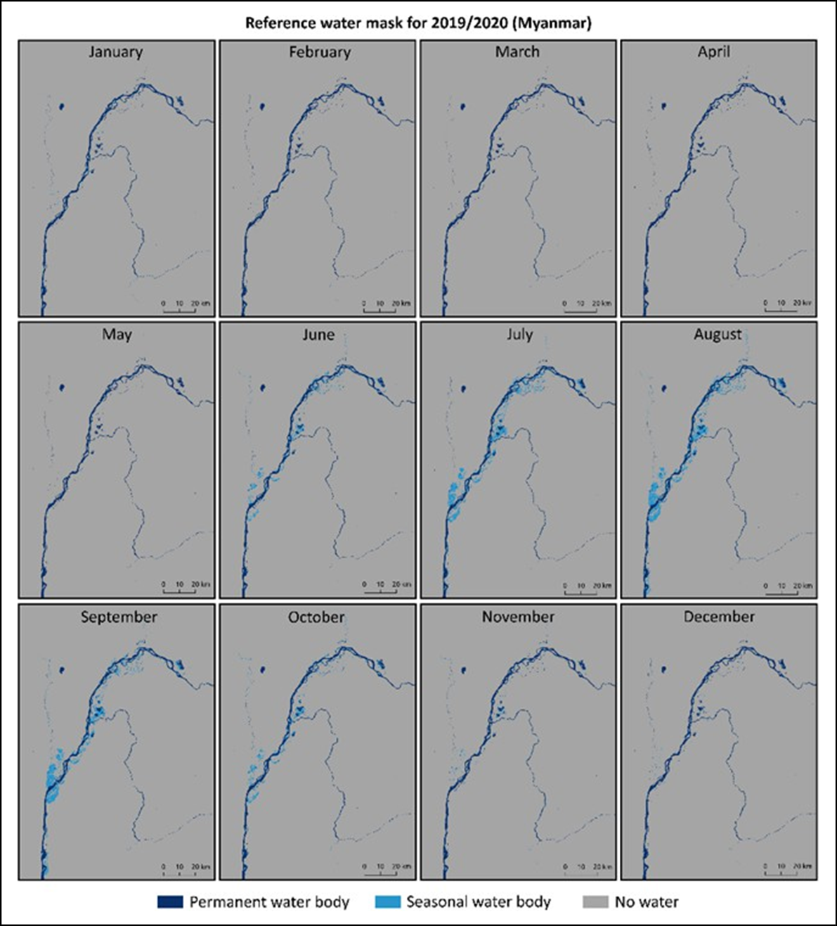
The GFM Reference Water Mask is a static dataset that is computed once for a reference period of five years, covering the years 2017 to 2021. A reference period of five years is chosen as a compromise, to have enough Sentinel-1 data for compuation, and to remove long-term hydrologic changes that might be integrated in the Reference Water Mask if longer time periods were used. Ending the reference period in 2021 is crucial to also include data from Sentinel-1 B.
The data values of the GFM Reference Water Mask are defined in Table 20.
| VALUE | DESCRIPTION | USER INTERPREATATION |
|
0 |
No water |
|
|
1 |
Permanent waterbody |
|
|
2 |
Seasonal waterbody (for thecurrent month) |
|
|
NaN |
No data available |
|
Table 20: Data values of the GFM output layer Reference Water Mask.
¶ 4.4 GFM output layer: Exclusion Mask
The identification of conditions under which the SAR-based flood mapping algorithms are deemed reliable, is an essential element of the GFM product, or indeed of any automated global flood monitoring system. This consideration is therefore an integral part of the near real-time flood detection and final preparation of the results of the GFM product.
The central assumption underlying the successful SAR-based identification and delineation of water bodies, and subsequently of flood extent, is the low backscatter signature of water surfaces. Under normal conditions, water surfaces observed by the Sentinel-1 SAR sensor show significantly lower backscatter values than surrounding areas, and the desired discrimination between water and non-water surfaces can be achieved with high accuracy and reliability. The inclusion of historical information stored in the backscatter “datacube” (time-series), which is a key element of the GFM product, provides additional discrimination criteria, further improving the GFM product’s reliability.
Nonetheless there are several surface types where SAR-based delineation of flood extent is hampered, or completely impeded. In order to prevent misclassification, such surface types are excluded from the flood mapping results, using the GFM Exclusion Mask. The GFM Exclusion Mask addresses static topography and land cover effects, where the interaction of C-band microwaves with the land surface is in general complex. In several situations flooded areas cannot be detected by Sentinel-1 SAR, over certain land cover types and terrain conditions, for physical reasons. The main surface types that are excluded from the GFM flood mapping results, are defined in Table 21.
| # | SURFACE TYPE | DESCRIPTION |
|
1. |
No-sensitivity: |
|
|
2. |
Water look-alikes: |
|
|
3. |
Topographic distortions (and low probability of flood occurrence): |
|
|
4. |
Radar shadow: |
|
|
5. |
Low Sentinel-1 coverage: |
|
Table 21: Surface types that are excluded from the GFM results using the Exclusion Mask.
The GFM Exclusion Mask is generated by combining sub-layers that address distinct physical and geometric effects, while ignoring permanent or seasonal water pixels from the reference water mask. In addition, no-data values from the Ensemble flood mapping algorithm indicate on a binary map grid-cells where SAR data could not deliver the information needed for robust flood detection.
Considering the complexity of the physical and geometrical effects described in Table 21, and their potential spatial overlaps and interactions, one combined Exclusion Mask is provided that is easy for users of the GFM product to interpret. The Exclusion Mask is based on offline-generated Sentinel-1 parameters and auxiliary thematic datasets. It is accessed in near real-time, and provided in addition to the other GFM product output layers. The necessary operations are done at the 20m-sampling of the Sentinel-1 preprocessed data cube. The methods used to generate the sub-layers of the GFM Exclusion Mask, corresponding to the surface types in Table 21, are described below.
¶ 4.4.1 GFM Exclusion Mask sub-layer: No-sensitivity areas
Floods in urban or vegetated areas are at risk of being missed alarms in terms of flood detection, as co-located flood extents potentially feature high instead of low backscatter. The formation of corner reflectors for the SAR microwaves through perpendicular buildings (urban) or plant stems (vegetation) over standing water surfaces leads generally to high backscatter and thus common SAR water mapping approaches fail in detecting water surfaces. Moreover, the detection of water-bodies under densely vegetated canopies is complicated by the absorption and diffuse scattering in the canopy itself, reducing the sensitivity to processes on the ground.
The no-sensitivity sub-layer of the GFM Exclusion Mask delineates all land cover types and areas where Sentinel-1 C-band SAR is not sensitive to flooding - or any other type of change - of the ground surface. These no-sensitive areas encompass both densely vegetated- and urban areas. In both cases, the loss in sensitivity reflects the fact that the Sentinel-1 signal is dominated by backscatter echoes from other parts of the observed scene.
In the case of vegetation, backscatter from the vegetation canopy increasingly dominates the signals coming from the ground for increasing biomass levels. Given the limited penetration capability of C-band waves, Sentinel-1 becomes essentially insensitive to flooding over high biomass areas such as forests and shrubland with biomass levels larger than 30-50 t/ha (Quegan et al., 2000). Backscatter from these high biomass land cover classes is in general rather stable and high, a feature that is often exploited in land cover classification schemes.
To identify densely vegetated areas, four parameters from the Sentinel-1 Global Backscatter Model (S1-GBM) were used: mean backscatter in VV (µ𝜎0𝑉𝑉 ) and VH (µ𝜎0𝑉H ) polarisation, mean cross polarisation ratio (µ𝜎0CPR , computed as VV/VH backscatter) and standard deviation in VH polarisation (𝑠𝑡𝑑(𝜎𝜎0𝑉H)) Locally variable thresholds (𝜏𝑖) were defined for each parameter to discriminate vegetated from not vegetated areas, with grid-cells classified as dense vegetation as follows:
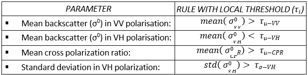
Thresholds were optimized separately per continent, and varied with northing and vegetation type. For the updated GFM product v3.x, the Global Forest Change dataset (Hansen et al., 2013; v1.10)5 was used as a reference dataset for threshold selection, and used directly as a dense vegetation mask in regions where irregular Sentinel-1 coverage caused artefacts (e.g. stripes of high and low backscatter) in the S1GBM layers. The global distribution of thresholds is shown in Figure 27.
Over urban areas backscatter measured by SAR C-band sensors is often dominated by comparably few, but very strong echoes received from buildings and other artificial objects (Sauer et al., 2011). The presence of large corner reflectors in form of buildings perpendicular to smooth horizontal ground create an extremely high backscatter signature, often close to saturation. Therefore, in the absence of sufficiently large open spaces between the buildings and urban vegetation, inundation in urban areas is difficult to detect. To identify the urban areas, in GFM v3.x products the GHSL R2023A E2018 data (at 10m)6 was used. The urban areas were defined as grid-cells where the GHS-BUILD value exceeds 35% probability of built-up area.
Finally, the dense vegetation mask and urban areas masks are combined with a logical “or” operation into one binary No-sensitivity mask.
¶ 4.4.2 GFM Exclusion Mask sub-layer: Water look-alikes
There is another situation where Sentinel-1 is not sensitive to the flooding of the ground, but for quite a different reason from that for vegetation and urban areas. Here the flood detection is challenged by non-water surfaces that have low backscatter themselves and would yield false alarms if not addressed. For example, very dry or sandy soils (e.g. on riverbanks or in deserts), frozen ground, wet snow and flat impervious areas (e.g. smooth tarmac such as airports, motorways, etc.) feature very low backscatter signatures and appear as water-look-alikes in SAR imagery.
In this case, the lack of sensitivity is due to the fact that backscatter from surfaces that are smooth (compared to the 5.5 cm wavelength of Sentinel-1’s C-band SAR sensor) can be as low as backscatter from a water surface. Smooth non-water surfaces may act like water as a specular reflector, scattering most energy of the SAR signal in forward direction, leading to very low backscatter values.
Separating water and smooth land surfaces based on a single SAR acquisition is hardly feasible. Therefore, the generation of a water look-alike sub-layer with permanent low backscatter is based on statistical information from Sentinel-1 time-series data. Grid-cells are masked if the occurrence of low backscatter values (below –15 dB) exceeds 70% of all values in the respective time-series. For the GFM product v3.x, the corresponding parameter baseline period for the determination of non-water low backscatter areas was set to 2020-2022, to reflect most recent conditions and to take into account recent land cover changes, e.g. ongoing desertification in arid regions.
¶ 4.4.3 GFM Exclusion Mask sub-layer: Topographic distortions
The consideration of local topography is essential for SAR-based flood detection in two ways. Firstly, there are areas that must be excluded during flood detection due to the geometry of the SAR observation. This is dealt using measures discussed in sub-Section 4.4.4 below. Secondly, SAR signal disturbances over areas of strong topography can be substantial, and can dominate the surface backscatter signature, and its change over time, leading to otherwise uncontrollable over- and under-estimation of flood extent. For this second case, consideration of the Height above Nearest Drainage (HAND) index is of vital importance to the reliability of the flood detection algorithms.
A binary Exclusion Mask, based on the HAND index (HAND-EM), has been calculated to separate flood- from non-flood prone areas, based on the elevation of each grid-cell to the nearest water-covered grid-cell (Twele et al., 2016; Chow et al., 2016). This is used as an input sub-layer of the GFM Exclusion Mask. Both binary classes are determined using an appropriate threshold value. A threshold value that is too high may lead to misclassifications (i.e. inclusion of flood look-alikes in areas much higher than the actual flood surface and drainage network). A threshold value that is too low may eliminate valid parts of the flood surface. Selecting an appropriate threshold is thus critical, and was carried out through a series of empirical tests including more than 400 Sentinel-1 and TerraSAR-X datasets of different hydrological and topographical settings (Twele et al., 2016).
Due to the global scope of the GFM product’s Sentinel-1 flood detection algorithms, a threshold value of ≥ 10 m was finally chosen to define non-flood prone areas. The HAND-EM has been further shrunk by one pixel using an 8-neighbour function to account for potential geometric inaccuracies between the exclude layer and the radar data. On a final note, since the Copernicus DEM is not hydrologically conditioned, the HAND index cannot be computed using this version of the DEM.
¶ 4.4.4 GFM Exclusion Mask sub-layer: Radar shadow
Radar shadow refers to areas that are unreachable by a radar signal, so no information can be gained. Radar shadow is a common effect in SAR imaging, appearing over strong terrain (especially at the far-range section of SAR images), and near high objects (e.g. mountains, high anthropogenic structures, forest borders). While the former are easily recognised with terrain and observation geometry analysis, the latter can only be identified using backscatter time-series, due to the global scope of the GFM product, and as real Digital Surface Models are only available for some areas.
The extent of radar shadow increases with radar range, so the far-range section of a SAR scene is more affected. After preprocessing, areas of radar shadow have very low backscatter values, so are likely to be confused with water surfaces, potentially leading to false alarms in flood detection. Two methods are used to provide radar shadow as one sub-layer of the GFM Exclusion Mask:
|
1 |
Statistical orbit-based approach: |
|
|
2 |
Geometric DEM-based approach: |
|
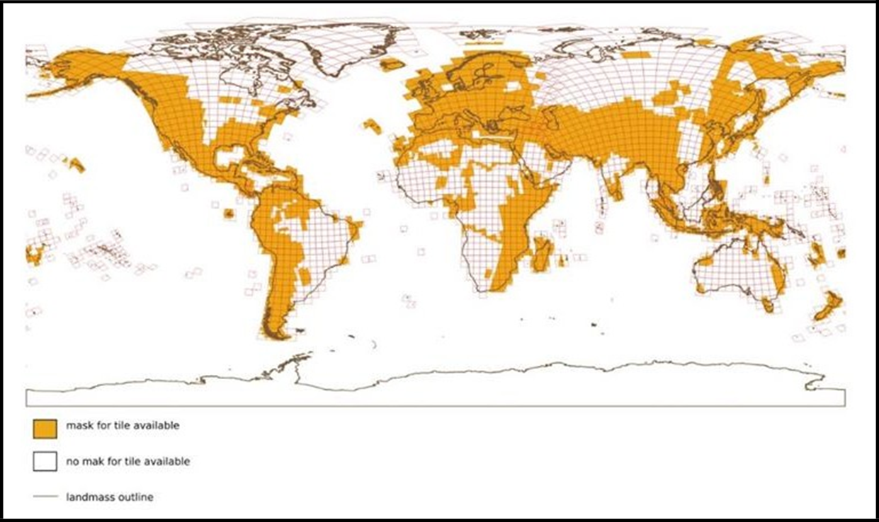
The orbit-based approach is well suited for masking radar shadow for the GFM product, as it models directly the backscatter signature of the Sentinel-1 observations. However it can only be used over areas with overpasses in both directions (i.e. ascending and descending). If one orbit direction is missing, this radar shadow mask cannot be produced. Figure 29 maps the global areas for which both directions are available, and where the orbit-based approach is used.
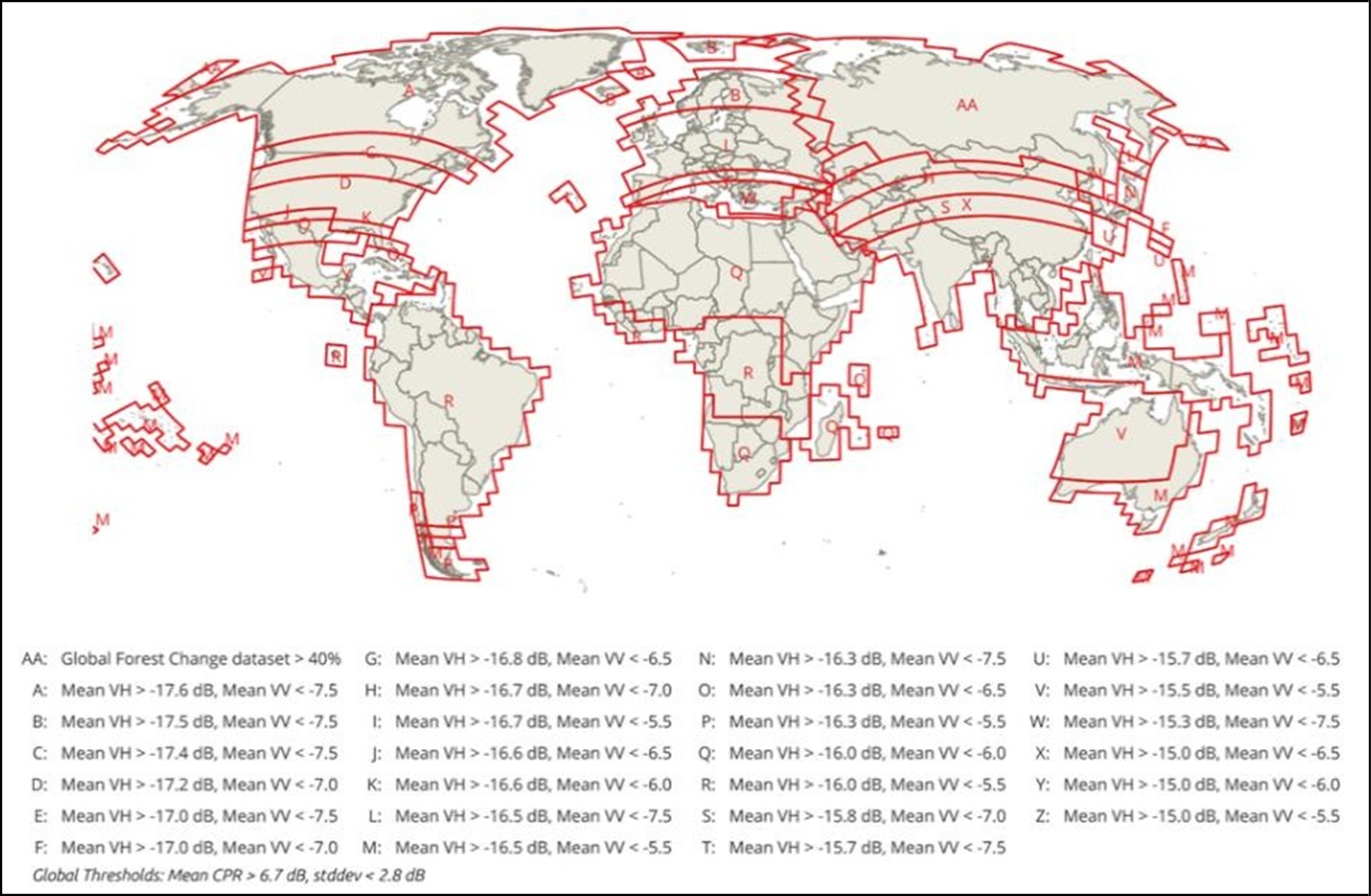
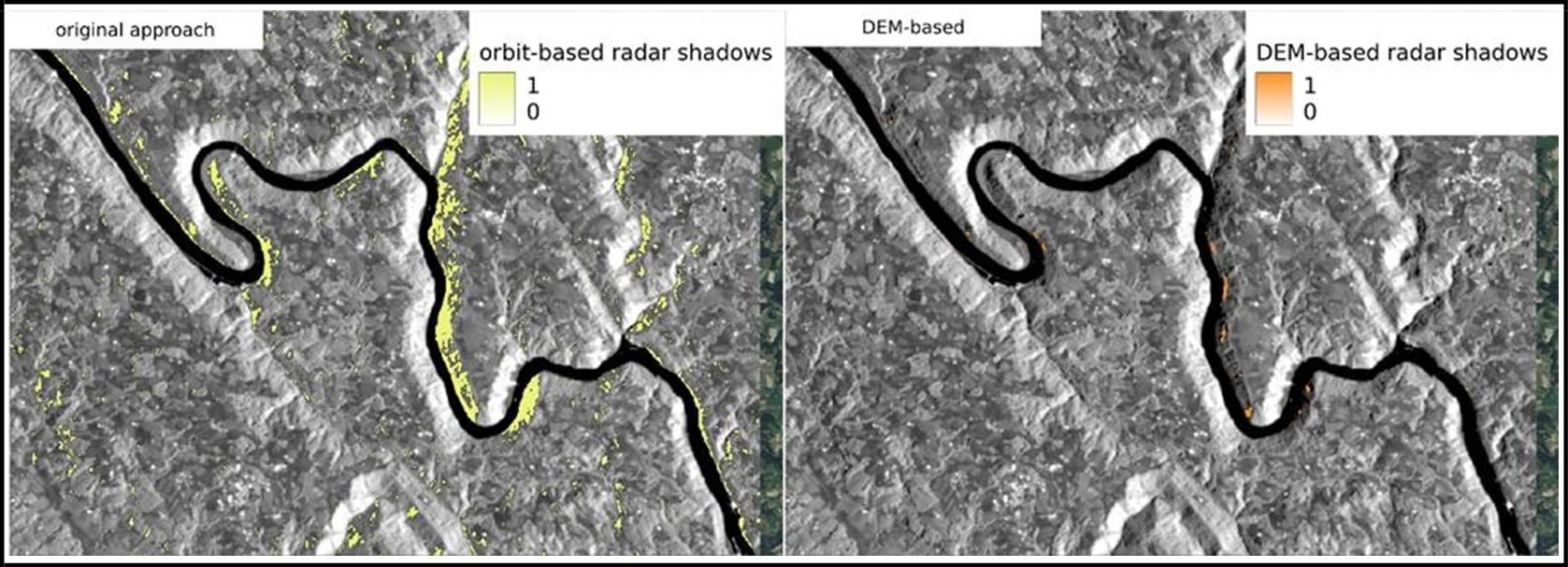
On the other hand, a DEM may only describe terrain elevation not surface elevation, or may have a too coarse a resolution to catch finer details. Thus it does not necessarily include anthropogenic structures or forests. The radar signal (at C-band) is mainly reflected at the surface leading to discrepancies with a terrain model. Therefore, a geometric observation model is not applicable for such smaller structures causing radar shadows, but delivers shadows caused by larger topographic features (e.g. mountains). The resulting differences between the two approaches can be seen in Figure 30. The combination of both methods in a single sub-layer allows for full coverage of all Sentinel-1 measurements, and the consideration of topography-related shadows, while shadows caused by finer details (e.g. forests) are considered only in areas of better Sentinel-1 coverage.
Consequently, both masking methods, the orbit-approach and the DEM-approach, are applied independently, and in a last step are joined to the final radar shadow masking. The join is done by logical “or” so that it is masked when at least one approach indicates a shadow configuration.
¶ 4.4.5 GFM Exclusion Mask sub-layer: Low Sentinel-1 coverage
In order to ensure high reliability of the results of the GFM product, areas where input data is insufficient and parameters and masks could not be produced, are also masked. This affects mainly the far North of Siberia and Canada due to poor or zero coverage by Sentinel-1, and lack of HAND-EM data. Furthermore, in response to erroneous Sentinel-1 images in the GFM data cube, a few tiles among the global land extent are masked, as no parameters or Exclusion Mask could be generated there. This is temporary safety measure in the initial project phase, and the low coverage layers are updated (i.e. reduced) on a regular basis to account for changes in the Sentinel-1 mission coverage, and the health of the GFM data cube. In particular, two low coverage input layers are used internally:
|
1 |
Low coverage on a pixel-level (LOWCOVPX): |
|
|
2 |
Low coverage on the T3-tile-level of the Equi7Grid (LOWCOVTILE): |
|
¶ 4.4.6 Global coverage of the input layers of the GFM Exclusion Mask
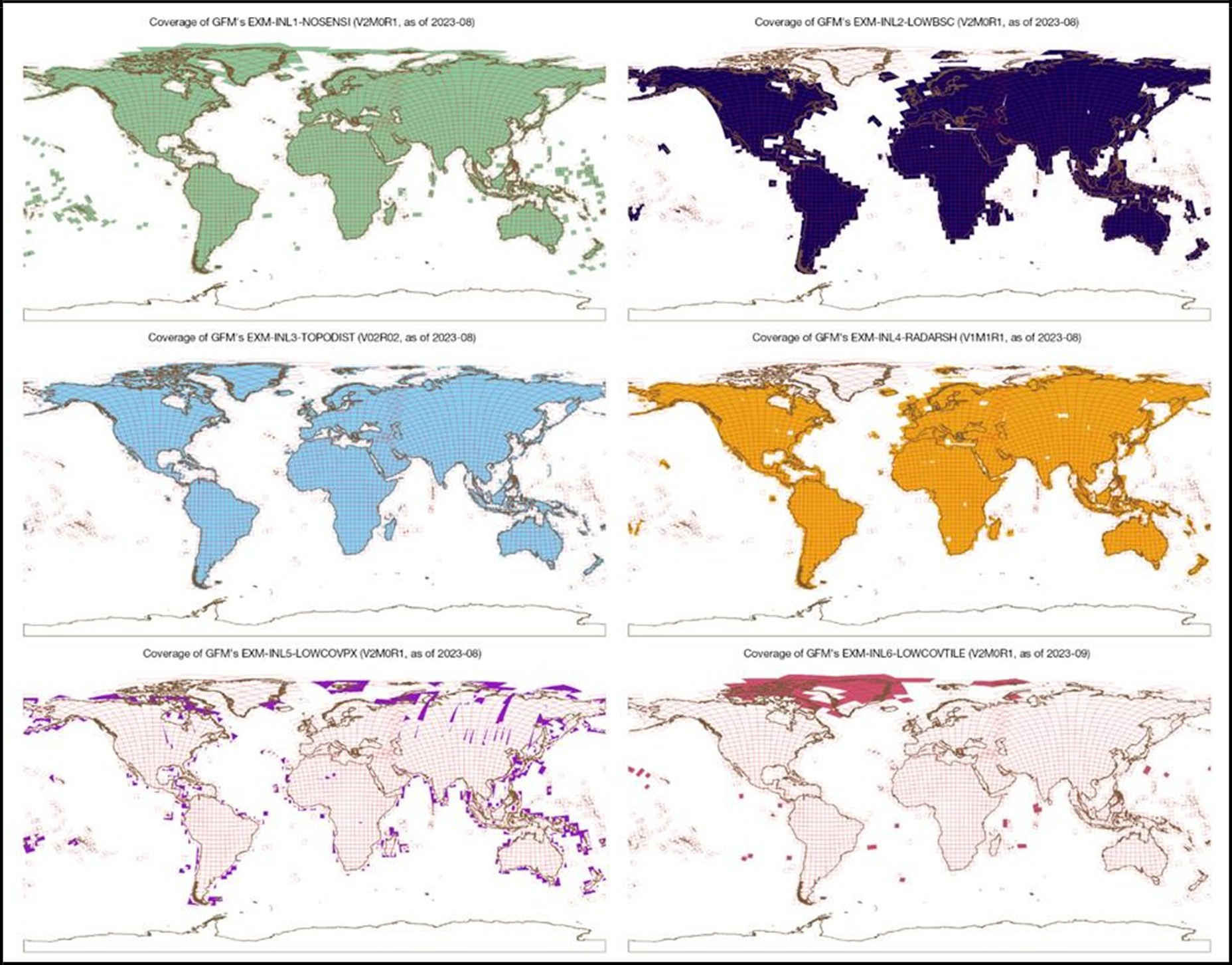
The Sentinel-1 and auxiliary datasets required for running the GFM product are not available everywhere. Figure 31 shows the global coverage of the GFM Exclusion Mask sub-layers. As can be seen, the global coverage of the GFM Exclusion Mask sub-layers can be summarized as follows:
- No-sensitivity masking (green) is globally applied.
- Non-water low-backscatter masking (dark blue) is applied quasi-globally (not in Greenland).
- Strong topography masking (light blue) is applied globally.
- Radar shadow masking (orange) is applied is most tiles.
- Pixel-level low Sentinel-1 coverage masking (violet) is done over scattered land areas in Asia, Africa, and North America.
- Tile-level low Sentinel-1 coverage masking (purple) is done over scattered areas in Asia, Africa, and North America over Arctic lands and islands.
¶ 4.5 GFM output layer: Likelihood Values
The GFM output layer Likelihood Values provides the estimated likelihood that is computed by the GFM Ensemble flood mapping algorithm, for all areas outside the GFM Exclusion Mask. In this context, the term likelihood represents flood classification accuracy for a given pixel. The methods used by the LIST, DLR, and TUW flood mapping algorithms to compute the Likelihood Values for a Sentinel-1 grid-cell, are described in Sections 3.1.5, 3.2.5 and 3.3.7, respectively. The method used by the GFM Ensemble algorithm to combine the Likelihood Values computed by the LIST, DLR and TUW algorithms, into a final Likelihood Value for each grid-cell, is described in Section 3.4.
Likelihood values lie in the interval [0, 100], where:
|
|
|
|
|
|
|
Finally, as mentioned in Section 3.3.7, the TUW flood mapping algorithm produces uncertainty values. In order to be used by the GFM Ensemble flood mapping algorithm, these uncertainty values have to be “flipped” so that low uncertainty values propagating towards 0 are remapped to high likelihood values propagating towards 100, and vice versa.
¶ 4.6 GFM output layer: Advisory Flags
Various meteorological factors may hamper or even prevent the detection of flooded areas. As discussed by Matgen et al. (2019), strong winds, rainfall, as well as the presence of wet snow, frost and dry soils are of particular concern. These factors are all important because they reduce the contrast between backscatter from open water surfaces and backscatter from the surrounding areas, thereby reducing the separability of flooded areas and surrounding land. While wind, frozen water surface and rainfall might reduce the backscatter contrast by increasing backscatter over water due to wind- and rainfall-induced roughening of the water surface, wet snow, frost and dry soils reduce the contrast by decreasing backscatter over the surrounding areas.
All of these deleterious effects are difficult to capture, due to their very dynamic nature and high spatial heterogeneity. Therefore, wind, rainfall, temperature, and snow data from sparsely distributed meteorological stations, and / or numerical weather prediction with its much coarser resolution, are hardly suited to capture the exact situation at the time of the Sentinel-1 acquisition, and are not ideal for providing the required advisory flags. While optical remote sensing satellites (e.g. MODIS, Sentinel-3) would provide sufficient spatial detail, optical data do not depict the environmental conditions shown by Sentinel-1, nor do they provide timely observations at all times, due to cloud cover and poor illumination conditions. Therefore, within the scope of the GFM product, microwave remote sensing data are the only robust and applicable source for environmental advisory flags. The applied approach is based on Sentinel-1 near real-time data and temporal parameters (see Section 3.1.2) derived from the Sentinel-1 data cube (time series) archive.
The purpose of the GFM output layer Advisory Flags is to raise awareness that meteorological conditions (wind, frozen conditions, etc.) may impair the detection of water bodies. As the Advisory Flags can only be retrieved at a coarser spatial resolution than Sentinel-1, this information is not forwarded to the Exclusion Mask. The Advisory Flags are provided as an additional layer, to guide users when interpreting the GFM results, allowing additional insight on local reliability at the time of Sentinel-1 acquisition. The Advisory Flags highlight grid-cells where SAR data may be disturbed by such processes during image acquisition, but the observed flood and water extents remain unmasked. In summary, grid-cells marked by Advisory Flags are not included in the Exclusion Mask, but users are advised to use with caution the observed water and flood extents for these areas.
The GFM Advisory Flags consist of two separate flaggings (i.e. for low regional backscatter and rough water surface), and are provided as four possible data values, as shown below:
| # | DEFINITION | USER INTERPRETATION |
|
0 |
|
High quality can be assumed. |
|
1 |
|
Caution advised, due to snow-covered, frozen, or dry soil affecting flood mapping reliability. |
|
2 |
|
Caution advised, due to local wind, rainfall, or frozen water surface affecting flood mapping reliability. |
|
3 |
|
Caution advised, due to both (a) snow-covered, frozen, or dry soil, and (b) local wind, rainfall, or frozen water surface affecting flood mapping reliability. |
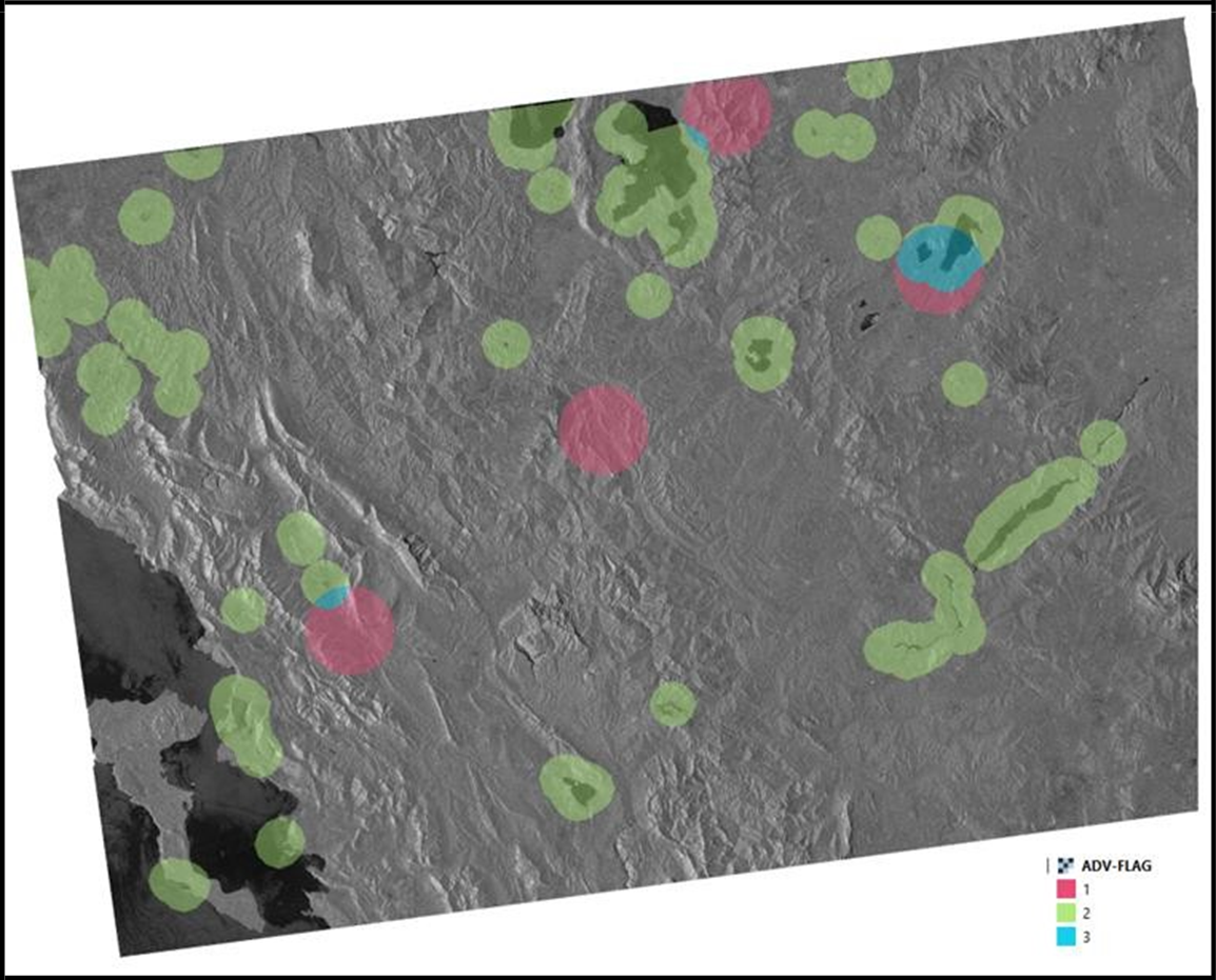
Figure 32 shows an example of the GFM Advisory Flags for a Sentinel-1 scene over Greece, acquired at a time when windy conditions where prevalent. In Figure 32, the Advisory Flags are overlaid on the backscatter image, with RED indicating low regional backscatter (i.e. snow, ice, or dryness), GREEN indicating rough water surface (i.e. wind, etc.), and BLUE indicating both conditions.
To generate the GFM Advisory Flags, it is necessary to combine the near real-time input data flow, with extracting the corresponding statistical parameters and auxiliary datasets. After processing the flood extent for the incoming Sentinel-1 scene, the Equi7Grid-tiles are identified, and the collocated parameters and auxiliary layers are read from the database. Figure 33 illustrates the data workflow, and how the flag values are set logically.
¶ 4.6.1 GFM Advisory Flags: Low regional backscatter
During the snow accumulation period, dry snow and ice-packs are almost transparent to microwaves. As a result, the SAR signal penetrates the snow / ice-pack up to several meters and the main contribution to the backscattering is from the snow–ground interface Rott et al. (1987). During the melting period, however, the increase of the amount of free liquid water inside the snow and ice bodies causes high dielectric losses, thereby increasing the absorption coefficient, featuring very low backscatter. In addition, the occurrence of meltwater puddles might change the backscattering behaviour of the surface, leading to components with specular microwave reflection, further decreasing the received amplitude at the sensor. Such patches of very low backscatter from those combined effects act easily as water-look-alikes and are source of false alarms.
Similarly, frozen soils with no free liquid water in the upper soil layers, show very low backscatter, appearing from the radar perspective as quasi-dry soils. Dried out soils are globally a more common issue for water and flood body detection, often showing backscatter values as low as calm water bodies. This ambiguity is hard to address, even with exploitation of time series analysis and statistical parameters, as the occurrence of dry soils is as erratic and unpredictable as flood events.
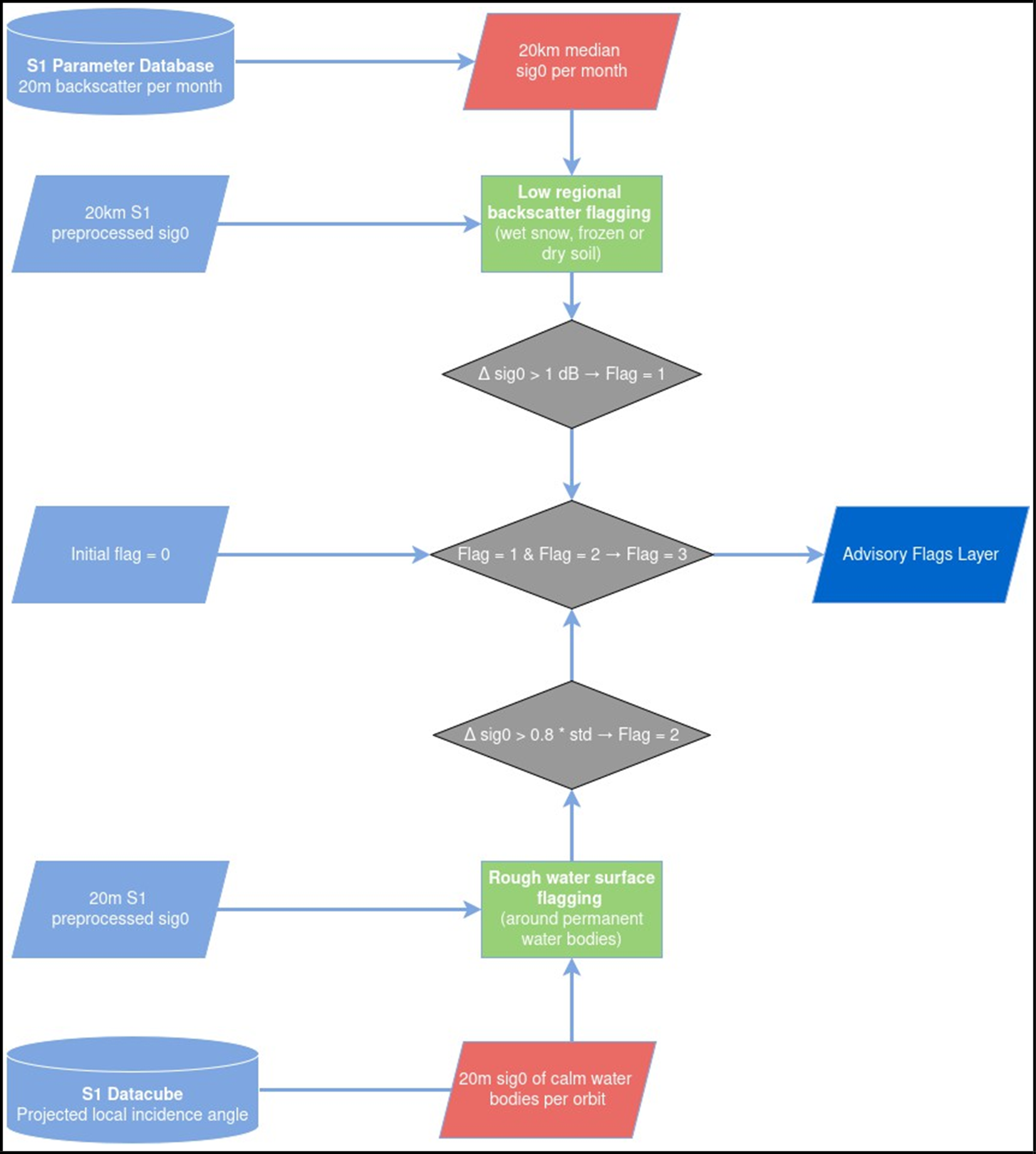
Low backscatter over large regions characterizes all the effects described above. Thus, to derive Advisory Flag 1 (low regional backscatter), the Sentinel-1 acquisitions are resampled to 20 km resolution, and the regional backscatter is compared to the regional monthly grouped median value (see Section 2.1.2) which represents seasonal backscatter signature of the corresponding region. Prior to resampling, each acquisition as well as the median image is masked using the Reference Water Mask (see Section 4.3), radar shadow mask (see Section 4.4.1.4) and the built-up area mask (see Section 2.2.5). The difference between regional backscatter and regional monthly grouped median backscatter reveals regionally low backscatter values that are likely to be caused by snow, frost or dry conditions while taking account of seasonal variations, such as annual changes in vegetation cover. If this difference exceeds 1 dB, the low backscatter flag is set to value 1, as follows:
- 𝒎𝒆𝒅𝒊𝒂𝒏(𝝈S1𝟎 ) > 𝝈S1𝟎 + 𝟏𝒅𝑩 → 𝑭𝒍𝒂𝒈 = 𝟏
These values are subsequently resampled to the 20m pixel sampling and a simple radial buffer of 14 km radius is applied to the identified pixels with regionally low backscatter. A known limitation of the used approach is the low number of flagged data in areas where frozen or dry conditions are typical for full months (e.g. permanently frozen soil during winter months in northern regions).
¶ 4.6.2 GFM Advisory Flags: Rough water surface
Wind, strong rainfall or frozen water surface over flood surfaces can lead to missed alarms, as they undermine the initial assumption of low backscatter due to specular reflection on smooth water surfaces. As a response to wind stress, short waves (of the order of centimetres to decimetres) are formed at the water surface causing an enhanced backscatter signal that occurs due to a constructive interference that reinforces the backscatter signal. This so-called “Bragg resonance effect” is dependent on wind speed and direction as well as on the radar wavelength.
For C-band SAR, the minimum threshold wind speed that can cause this effect and thus enhance the backscatter from water surface is estimated to be 3.3 m/s. Similarly, strong rainfall events roughen the water surface and thus lead to the enhanced backscatter. In case of the frozen lake surface, the enhanced backscatter values are caused by the scattering from water / ice transitions. For the detection of these effects, we make use of the backscatter signature of permanent water bodies inferred from time series within the Sentinel-1 data cube archive.
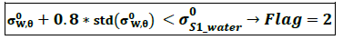
The near real-time 20m Sentinel-1 backscatter data over the areas identified by the GFM Reference Water Mask (see Section 4.3) and additional criteria based on backscatter, are analysed. For the grid-cell to be identified as water and used for setting the rough water surface flag, it must to be identified as permanent or seasonal water by the Reference Water Mask for the given month, has to have backscatter value below –10 dB and deviate from the expected calm water signature. The criteria based on backscatter are needed, as the water bodies shape might deviate from the seasonally defined reference water mask. For this reason, masking of very high backscatter values helps to avoid setting the rough water surface flag due to the changed water body shape instead of roughening of its surface. Additionally, an erosion step is applied to the selected water bodies, to remove false positives in shallow waters at the water borders.
Over the identified water pixels, a check is made of whether the backscatter deviates from a calm water signature. In the case of a rough water surface, there is most likely an increased backscatter indicative of strong winds, rainfall, or frozen water surface, which in turn are likely to increase the backscatter from the nearby water surfaces also over the flooded areas.
For the calm water signature, we chose the linear water backscatter model 𝛔𝟎W𝛉 dependent on the project local incidence angle 𝜃 (see Section 3.3.1) and also used in the TU Wien algorithm (see Section 3.3) as baseline. An analysis of backscatter images at windy conditions showed the suitability of the water backscatter model’s standard deviation (𝐬𝐭𝐝(𝛔𝟎W𝛉)) to distinguish rough from non-rough water surfaces, with respect to the local calm water signature.
On the condition that this limit is exceeded over water surface, we set, on the 20m pixel scale, the rough water surface flag to value 2, as follows:
Finally, all grid-cells identified as roughened permanent water bodies are spatially filtered using morphological operators. Assuming that wind, rainfall or frozen water surface effects are highly correlated within the neighbourhood, a simple L2/radial buffer of 5km radius is applied to the identified rough water surface grid-cells, effectively enlarging the identified area.
All pixels within the buffered area are labelled with Advisory Flag 2 (rough water surface). This should also reflect the initial expectation that the majority of floods appear in the vicinity of rivers and permanent or seasonal water bodies, and the wind flag is needed by users in those areas.
It should be noted that this realisation of the wind flag constitutes the current version in the GFM product. Some tweaking and optimisation towards the alert accuracy, is forseen, as more experience with the operational service is gained.
Finally, the 20m pixel array for the Advisory Flag is obtained from the combination of both intermediate flag outputs. All pixel locations that have values in the incoming Sentinel-1 image are initiated with value 0, and are updated with the following operation (which effectively sets to value 0 all grid-cells with no flag set, and sets to value 3 all grid-cells where both flags are set)

Note that a known limitation of the applied approach is that flags issued due to land cover change (e.g. changed shape of water body compared with the Reference Water Mask, with the resulting enhanced backscatter misinterpreted as roughened water surface). Generally, the quality of this flag is strongly dependent on the quality and timeliness of the Reference Water Mask.
¶ 4.7 GFM output layer: Sentinel-1 Footprint and Metadata
The GFM output layer Sentinel-1 Footprint and Metadata includes all available metadata (i.e. acquisition parameters) provided with each Sentinel-1 GRD image processed by the GFM product. The metadata for each Sentinel-1 GRD scene is provided in the distributed Sentinel SAFE (Standard Archive Format for Europe) format included in the “manifest.safe” file. This is an XML file containing the mandatory product metadata. Attributes in the manifest file are classified into four categories:

Platform and instrument related attributes are considered as static for the different Sentinel-1 satellites. A total number of 29 attributes are contained in the manifest file, including information about the absolute orbit number, pass direction, polarisation, sensing start and end date and the product timeliness category. A summary of the included attributes is shown in Table 22.
The footprint of a Sentinel-1 GRD scene, as provided in each data product, is included in the aforementioned manifest file. The footprint is represented as a human readable JTS (Java Topology Suite) object named “JTS footprint”. The JTS footprint is converted into Well-known Text (WKT) and Well-known Binary (WKB) in the process of parsing and ingesting the acquired manifest files into the operated metadata database. WKT and WKB are originally defined by the OGC (Open Geospatial Consortium) to describe simple features. On-the-fly conversion to GeoJson is provided to aggregate the requested footprint features into the corresponding layer request by the user.
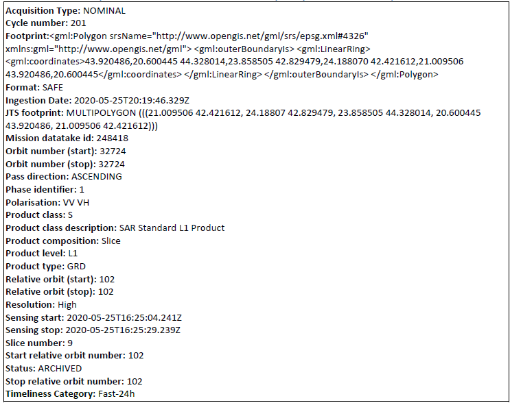
Table 22: Example of metadata fields in the GFM output layer Sentinel-1 Footprint and Metadata.
¶ 4.8 GFM output layer: Sentinel-1 Schedule
Sentinel-1 observations follow a strict acquisition planning often referred to as acquisition segments. Information on the planned future acquisition is provided by ESA in form of KML files. A single file usually covers an acquisition period of about 12 days, with the start and stop time of the future planned acquisitions already given in the file name. KML files are publish by ESA on a regular base, well before activation, with potential last-minute changes due to requests from CEMS. Information in the KML files is organized based on planned data takes.
The parameters included in the KML file are listed in Table 23. KML files are regularly checked, downloaded and ingested into the metadata database for further analysis. All parameters are available for requesting the schedule information indicating the next planned Sentinel-1 GRD acquisition for a given location.
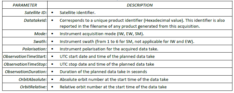
Table 23: Information in the GFM output layer Sentinel-1 Schedule, indicating the next planned Sentinel-1 GRD acquisition.
¶ 4.9 GFM output layer: Affected Population
The GFM output layer Affected Population provides information about the flood-affected population, which is extracted from the Global Human Settlement Layer (GHSL) of CEMS, in particular the GHS-POP dataset. This data contains a raster representation of the population’s distribution and density, as the number of people living within each grid cell.
The information is available at various spatial resolutions and for different epochs. The GFM product uses the dataset at the highest possible (250m) resolution and for the latest available time-step, (2015). The dataset has been re-projected to the same grid system as the flood map, i.e. the Equi7Grid with a 20m pixel spacing and 300km gridding (T3 level), and resampled to 20m resolution.
¶ 4.10 GFM output layer: Affected Land Cover
The GFM output layer Affected Land Cover provides the land cover information which is extracted from the Copernicus Land Monitoring Service, making use of the Global Land Cover dataset, available at a global level at 100m resolution. The Copernicus Global Land Cover (3) includes 23 classes and provides annual updates. The dataset was reprojected to the same grid system as the flood map itself, which is the Equi7Grid with a 20m pixel-spacing and a 300km gridding (T3 level). The data was then resampled from 100m to 20m resolution. This information provides a first assessment of affected land cover or land use types, such as how much agricultural area is affected by flooding within the GFM Observed Flood Extent or the area of interest.