The DLR flood mapping algorithm makes use of an automatic hierarchical tile-based thresholding approach in combination with a fuzzy logic-based post-processing step for the unsupervised extraction of the flood extent in Sentinel-1 SAR data. The algorithm consists of three steps:
- unsupervised initialization of the water classification by hierarchical automatic tile-based thresholding, to derive a global threshold backscatter value between water and non-water
- fuzzy logic-based refinement of the initial water classification, in order to exclude water look-alikes, using SAR backscatter values, topographic slope, and the size of detected water bodies
- region growing of the defuzzified water classification, in order to integrate the transient shallow water zone between flooded and non-flooded areas
The DLR flood mapping algorithm requires the followingfour main input raster datasets:
|
|
|
|
Initial descriptions of the DLR flood mapping algorithm are provided by Martinis et al. (2015) and Twele et al. (2016). The main steps of the DLR flood mapping algorithm are described below.
¶ 3.2.1 Unsupervised initialization of water classification by tile-based thresholding
In the first stage of the DLR flood mapping algorithm an automatic, parametric tile-based thresholding procedure is applied to the Sentinel-1 SAR image scene, to derive a global threshold backscatter value between water and non-water classes. The global threshold is calculated for a selected limitednumber of representative image subsets (or tiles), and is then applied to the entire image scene by labelling as “water” all pixels with backscatter values lower than the threshold.
The selection of representative tiles for calculating the global threshold backscatter value is based on the assumption that tiles with low mean backscatter values and high standard deviations, have bimodal backscatter distributions and are likely to contain both water and non-water features.
This first step of the DLR flood mapping algorithmis carried out in two stages, as described below:
- selection of tiles containing bimodal backscatter distributions and water-land boundaries
- calculation of the optimalglobal threshold backscatter value separating water and land
¶ 1. Selection of tiles containing bimodal backscatter distributions and water-land boundaries:
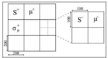
In the first stage of step1 of the DLR flood mapping algorithm, a two-level quadtree data structure is generated which, at the first or parent level (denoted as S+), splits the SAR image scene into a discrete number of non-overlapping image subsets (called parent tiles), each ofdefined size C by C pixels (where C = 200).
Each parent tile is represented at the second or child level (denoted as S-) by foursquare sub-tiles, each of size C/2 by C/2 pixels.
The two-level quadtree-based splitting of a SAR image by the DLR flood mapping algorithm, is illustrated in Figure 5.
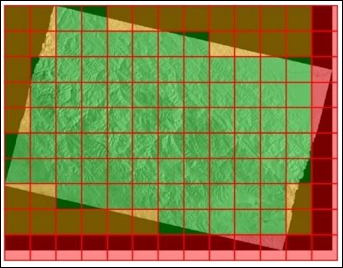
To determine the global threshold backscatter value between water and non-water, representative parent tiles are selected based on the probability (determined by the statistics of their backscatter values) that they contain a bimodal mixture of water and non-water pixels. The following situations (illustrated in Figure 6) can result in parent tiles that are not valid for threshold calculation:
|
|
|
The statistical parameters and procedure used to select representative parent tiles that most likely contain bimodal backscatter distributions and water-land boundaries, are described in Table 13.
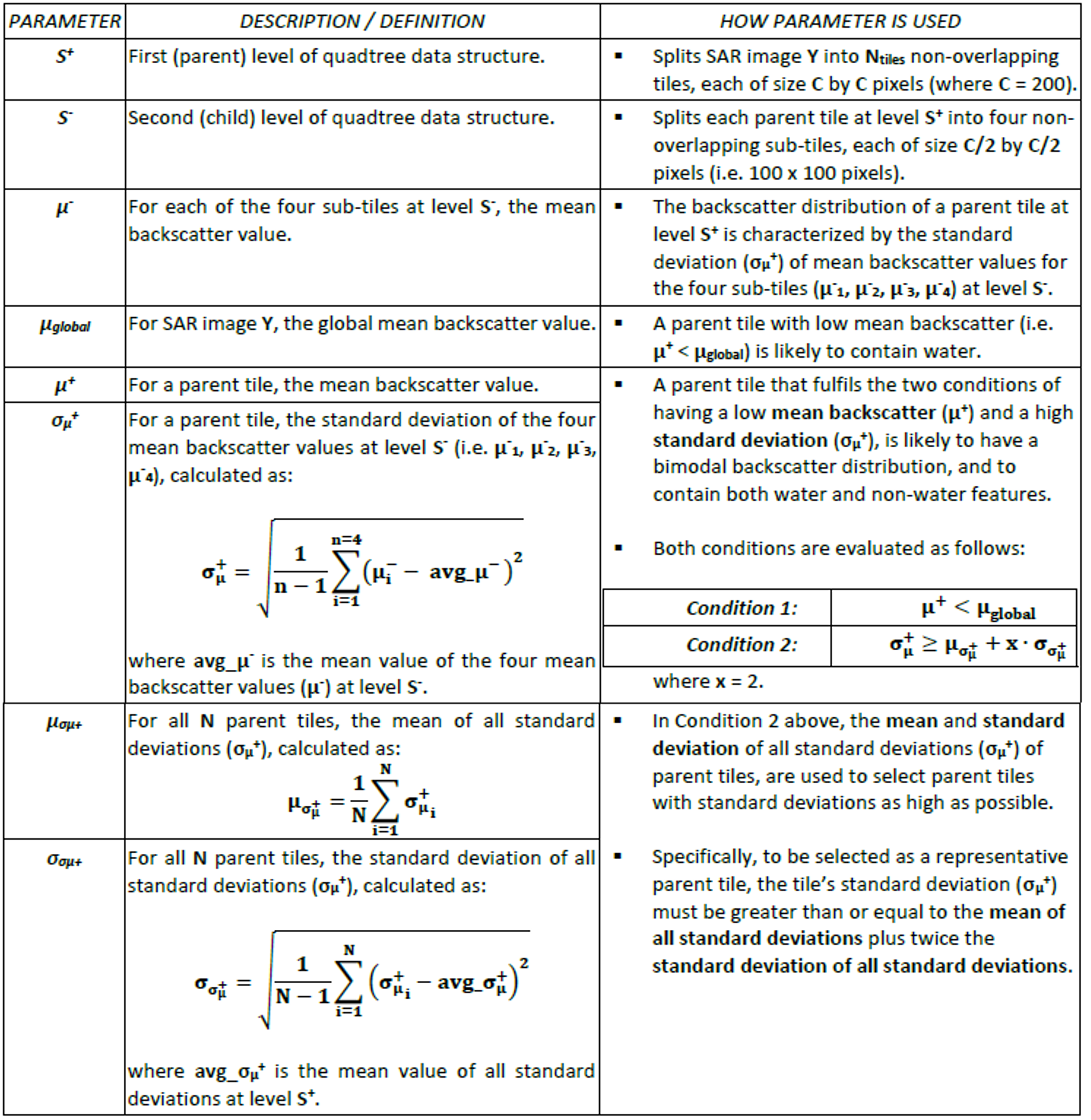
Table 13: Summary of the statistical parameters and procedures used to select representative parent tiles likely to contain bimodal backscatter distributions and water-land boundaries.
As is described in Table 13, in order to be selected as a representative image subset, a parent tile (i.e. at level S+in the quadtree) must fulfil two conditions:
|
Condition 1: |
|
|
Condition 2: |
|
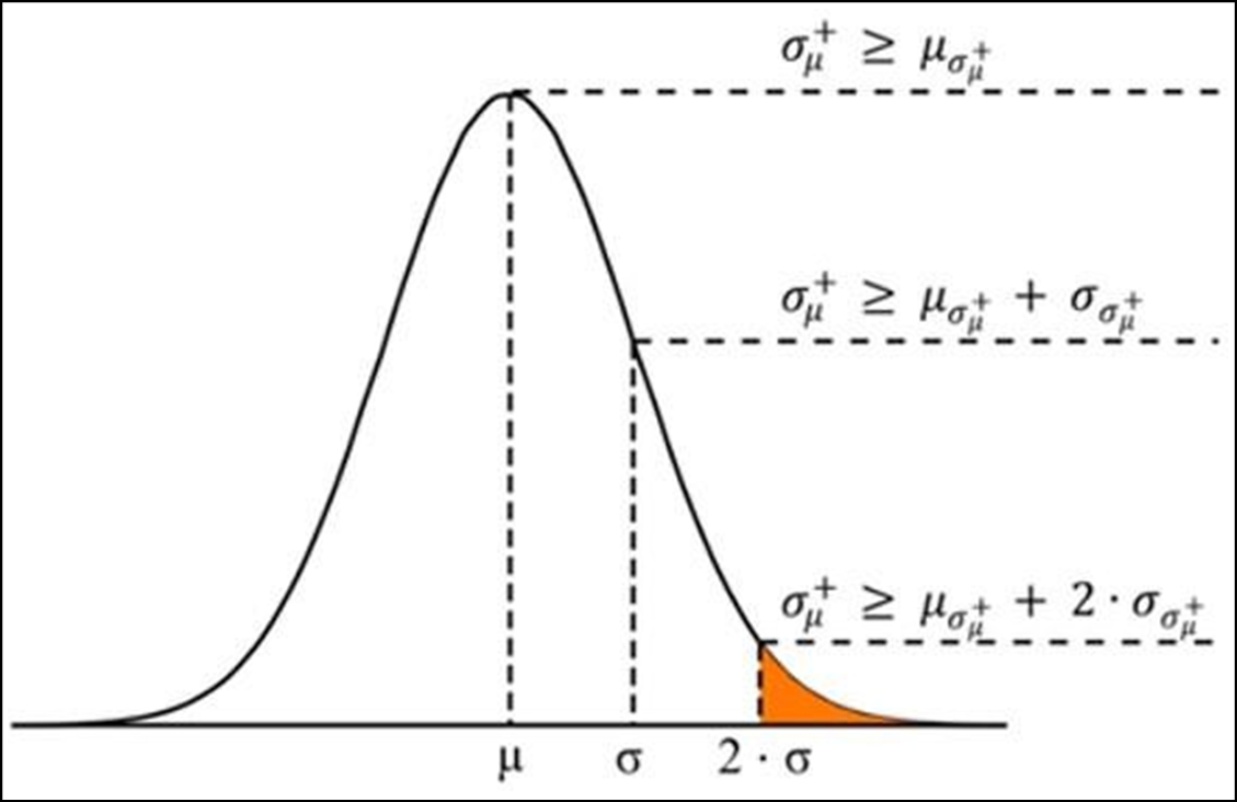
Specifically, in order to fulfil Condition 2, a parent tile’s standard deviation (σµ +) must be greater than or equal to the mean of all standard deviations plus twice the standard deviation of all standard deviations. This concept is illustrated in Figure 7, where all standard deviations (σµ +) are plotted into a Gaussian distribution. As can be seen, a standard deviation (σµ +) greater or equal to the distribution’s mean, or even the mean plus one standard deviation, would still leave too many parent tiles, the majority of which may not show bimodal backscatter distributions.
Once the sample of representative parenttiles most likelyhaving bimodal backscatter distributions and water-land boundaries is selected (using Conditions 1 and 2), the following checks are made:
- if the number of selected representative parent tiles is insufficient (i.e. only 10 or less), a bigger sample is obtained by re-applying Conditions 1 and 2 (see Table 13), with an increased range of allowed standard deviations (i.e. set x = 1.28, instead of x = 2)
- if more than 10 representative parent tiles have been selected, a statistically-sound sample of representative parent tiles is assumed. The five representative parent tiles with the highest backscatter standard deviations (σµ +) are then used for further threshold computation
¶ 2. Calculation of the optimal global threshold backscatter value separating water and land:
All of the representative parent tiles that are selected as described above are likely to contain bimodal backscatter distributions and valid water-land boundaries, as illustrated Figure 8 below.
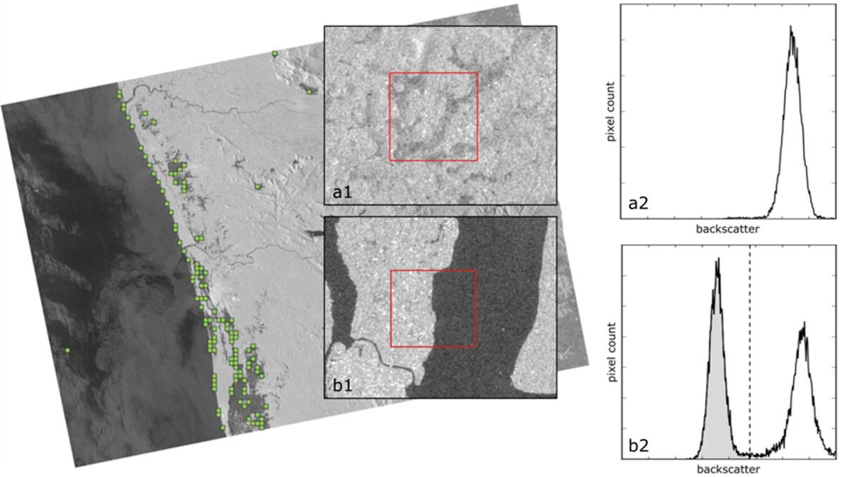
In order to derivethe optimal globalthreshold backscatter value between the water and non-water classes (indicated in panel b2 of Figure 8), the automatic, histogram-based thresholding method of Kittler and Illingworth (1986) is applied to the five representative parent tiles with the highest backscatter standard deviations (σµ +).
This method (calledthe minimum error thresholding or MET method) is an iterative, cost-minimization approach that splits the histogram into two classes with a threshold that identifies the class boundary. (Note that Otsu’s method of histogram thresholding, which is used in the LIST flood mapping algorithm, is a special case of the MET method).
The optimal global threshold backscatter value (τ) separates both classes with minimum effort. As can be seen in Figure 8, if selecting a pure land tile (panel a1), the corresponding histogram (panel a2) is unimodal. If selecting a tile with both low and high backscatter values (panel b1), the corresponding histogram (panel b2) is bimodal, and we assume a water-land-boundary.
If applying a threshold to the latter histogram, both classes can be separated, giving the class water in the left part. The final global threshold backscatter value (τ) is obtained as the mean of the threshold values (τ+) of the five individual representative parent tiles. Applying this threshold to the entire Sentinel- 1 SAR image scene results in an initial water classification.
In addition to the optimal global threshold backscatter value (τ) separating water and non-water, we also compute the mean backscatter value of the water class (µwater), as this is used in the fuzzy logic-based refinement of the initial water classification (as described in Section 3.2.2 below). In accordance with Kittler and Illingworth (1986), we compute the mean backscatter value of the water class (μwater) as the geometric centroid of the separated class in the histogram, as follows:
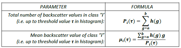
where:
Class “i” refers to the water class.
- τ is the global threshold backscatter value separating water and non-water
- a is the minimum backscatter value in class“i”
- b is the maximum backscatter value in class“i”
- g is the backscatter value of a histogram bin
- h(g) is the histogram count of backscatter value “g”
As was done for calculating the global threshold backscatter value (τ), the mean backscatter value for water (μwater) for the entire Sentinel-1 SAR image scene is calculated as the average of the mean backscatter values for water derived for the five representative parent tiles.
Finally, if the automatic tile-based histogram thresholding fails to compute a reliable global threshold backscatter value (τ), or returns an unusually high value (i.e. τ > -15 dB) for a representative parent tile, a fallback threshold mechanism is activated. This fallback system determines thresholds individually for each Sentinel-1 scene by analysing backscatter values from known inland water bodies, identified in the Copernicus Water Body Mask (see Section 2.2.3).
Empirical testing has established that the 60th percentile of backscatter values from these inland water bodies provides a suitable fallback threshold when it falls between -20 dB and -16 dB. If this calculation fails, the system implements a graduated response, as follows:
- default value of -18 dB, if calculation completely fails
- value of -19 dB, if calculated fallbackthreshold falls below -20 dB
- value of -17 dB, if calculated fallbackthreshold exceeds -16 dB
The global threshold is reset to these fallback values when at least two parent tiles require fallback thresholds and the fallback value is lower than the mean threshold across the five parent tiles. To prevent underestimation, this reset mechanism is not triggered when all originally determined thresholds are consistently high (and therefore likely accurate).
¶ 3.2.2 Fuzzy logic-based refinement of the initial water classification
In the second stage of the DLR flood mapping algorithm, a fuzzy logic-based approach is used to refine the initial water classification that was derived by applying the global threshold backscatter value between water and non-water (τg) to the Sentinel-1 SAR image. The objective is to improve the thematic accuracy of the initial water classification, by removing potential water look-alikes.
In the fuzzy logic-based approach, the likelihood of a SAR image pixel being classified as water is determined by its degree of membership to the water class, ranging from 0 (not belonging) to 1 (completely belonging). For each pixel, the degree of membership to the water class will be low if:
a) the pixel has a high backscatter value, close to the global threshold backscatter value (τg)
b) the topographic slope at that pixel is high, since steeper surfaces are unlikely to retain water
c) the pixel has a low number of neighbouring water pixels, since dispersed small areas of low backscatter are commonly related to water look-alike areas.
Conversely, a pixel’s degree of membership to the water class will be high if the pixel has a low backscatter value, low topographic slope and a high number of neighbouring water pixels.
To computethe degrees of membership to the water class (or fuzzy values) of SAR imagepixels, the Standard Z or S fuzzy membership functions(see below) are applied to three input datasets: (a) the backscatter values (σ0) in the Sentinel-1 SAR image; (b) topographic slope, computed from the DEM; and (c) the size of individual water bodies in the initial water classification.
To compute the degrees of membership to the water class (or fuzzy values) of SAR image pixels, the Standard Z or S fuzzy membership functions (see below) are applied to three input datasets: (a) the backscatter values (σ0) in the Sentinel-1 SAR image; (b) topographic slope, computed from the DEM; and (c) the size of individual water bodies in the initial water classification.
The Standard Z and S fuzzy membership functions are illustrated in Figure 9. The Standard Z fuzzy membership function (or Negative S-function) assigns higher degrees of membership (fuzzy values) to lower input pixel values, and lower fuzzy values to higher input pixel values. The Standard S fuzzy membership function (or Positive S-function) does the opposite, assigning lower fuzzy values to lower input pixel values, and higher fuzzy values to higher input pixel values. As can be seen, for both fuzzy membership functions the range of input pixel values is specified by the lower and upper threshold values (a and c, respectively), with a cross-over point (b) defined as b = (a + c) / 2.
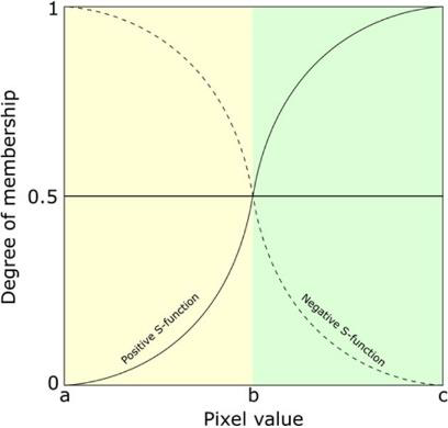
In our case, since low degrees of membership to the water class are associated with both high backscatter values and high topographic slope, we apply the Standard Z fuzzy membership function to the input datasets of backscatter values and topographic slope, in order to compute the fuzzy values for both datasets. Conversely, since high degrees of membership to the water class are associated with high numbers of neighbouring water pixels, we apply the Standard S fuzzy membership function to the input dataset of size of individual water bodies.
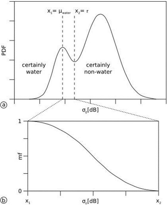
Figure 10 illustrates the application of the Standard Z fuzzy membership function to discriminate between water and non-water, based on backscatter values (σ0) in the Sentinel-1 SAR image. As can be seen in Figure 10, the range of input backscatter values for the fuzzy membership function is specified by the lower and upper threshold values (X1 and X2), which are defined as follows:
| Lower fuzzy threshold value (X1): |
|
| Upper fuzzy threshold value (X2): |
|
The upper and lower fuzzy threshold values that are used for applying the Standard Z and S fuzzy membership functions to compute the fuzzy values for the input datasets of backscatter values, topographic slope, and size of individual water bodies, are summarised in Table 14.
|
INPUT VARIABLE |
FUZZY MEMBERSHIP FUNCTION | LOWER FUZZY THRESHOLD VALUE (X1) | UPPER FUZZY THRESHOLD VALUE (X2) |
|
Backscatter values(σ0) |
Standard Z |
Mean backscatter value (μwater) of water pixels | Global threshold value (τg) between water andnon-water |
|
Topographic slope |
Standard Z |
0 degrees |
18 degrees |
|
Size of individual waterbodies |
Standard S |
10 pixels |
500 pixels |
Table 14: Upper and lower fuzzy threshold values (X1 and X2) used to compute the degrees of membership to the water class, for the input datasets of backscatter values, topographic slope, and size of individual water bodies.
The result of applying the fuzzy logic-based approach to the three input datasets is a fuzzy set consisting of three layers (one for each variable) of degrees of membership to the water class (i.e. the fuzzy values), with floating point values in the range [0, 1]. For performance reasons, the fuzzy values are rescaled to the range [0, 100]. The three fuzzy layers are combined into a single layer of fuzzy values by calculating, for each pixel, the mean of the three degrees of membership to the water class. In the final step of the fuzzy logic-based approach, a defuzzified water classification is created, by labelling all pixels with a mean fuzzy value ≥ 0.6 as correct water classifications.
¶ 3.2.3 Region growing of the defuzzified water classification
The transient shallow water zone between flooded and non-flooded areas is often characterized by successively increasing backscatter levels, mainly due to a higher signal return of emerging vegetation. The objective of the region growing step of the DLR flood mapping algorithm, is to integrate these areas in the flood classification, and to increase the spatial homogeneity of the detected flood plain. The following three input datasets are used as input for the region growing:
- the single layer of fuzzy values showing the mean degrees of membership to the water class.
- the defuzzified water classification, showing all image pixels with a mean fuzzy value ≥ 0.6.
- a dataset showing the size (in pixels) of the water regions (i.e. sets of connected water pixels) in the defuzzified water classification.
The region growing is implemented in two stages, which are described as follows:
|
1 |
Selection of seedpoints: |
|
|
2 |
Tolerance for region growing: |
|
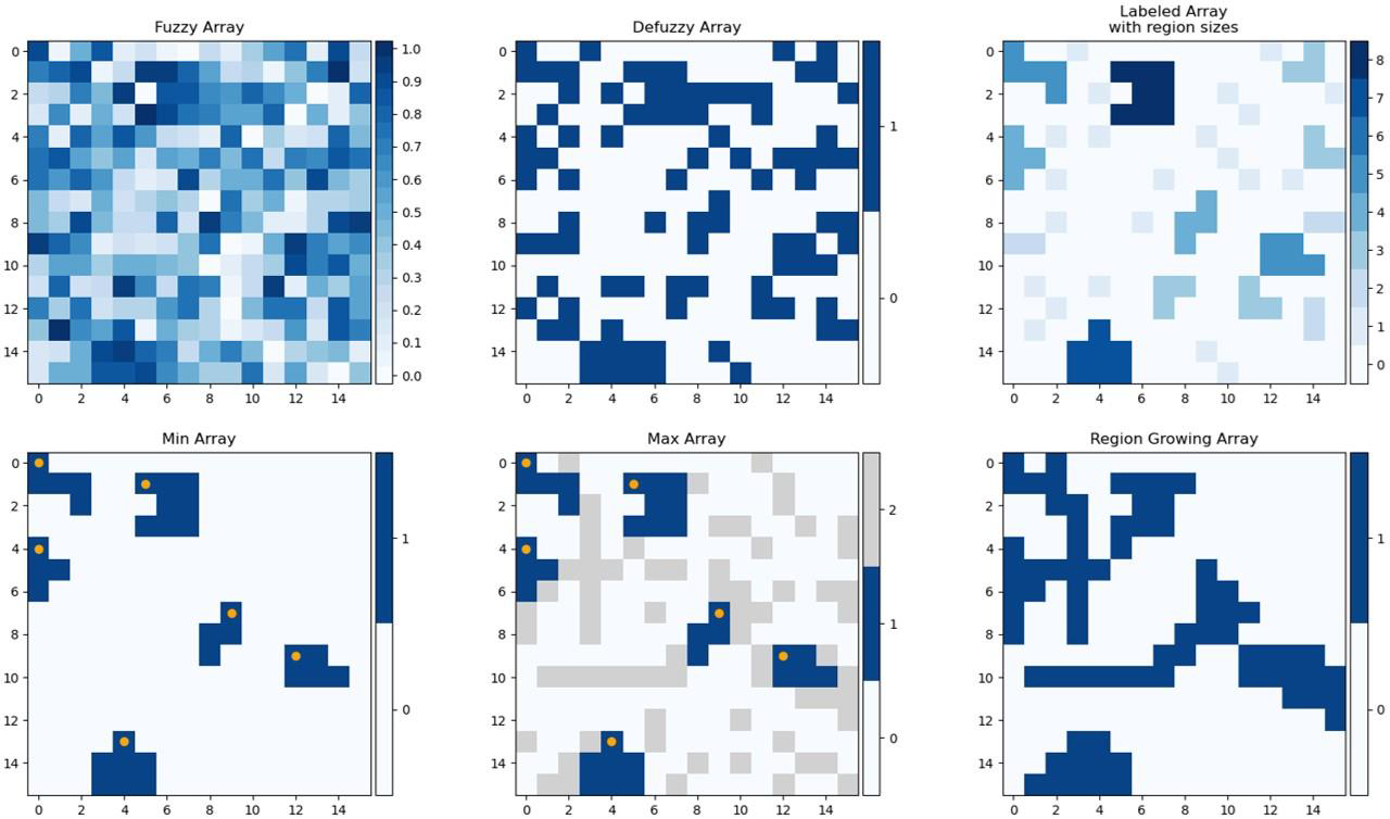
The implementation of the region growing step for a 16x16 pixel sub-image is illustrated in Figure 11, where the contents of the six arrays shown are described below:
|
1 |
Fuzzy Array: |
|
|
2 |
Defuzzy Array: |
|
|
3 |
Labelled Array with region sizes: |
|
|
4 |
Min Array: |
|
|
5 |
Max Array: |
|
|
6 |
Region Growing Array: |
|
¶ 3.2.4 Final post-processing of the DLR flood map
Any small fragmented patches of the water and non-water classes in the region growing results are first eliminated using a blob removal method, which is implemented as follows:
|
|
An additional region growing operation is performed, based on the SAR backscatter values, to include directly connected pixels that are within a tolerance criterion of 1 decibel (dB). In contrast to the previous steps, the parameters for this region growing are determined by the algorithm, and cannot be static. The region growing is implemented in two stages, as described below.
|
1 |
Selection of seed points: |
|
|
2 |
Tolerance for region growing: |
|
Finally, it should be noted that before the DLR flood mapping algorithm is implemented, the input Sentinel-1 SAR backscatter values are rescaled from the original range (-40 - 0 db) to 0 - 400, to ensure positive input values for all processing steps. Thus, the additional region growing operation, for example, is implemented using rescaled backscatter values, as shown below:
| Backscatter values(dB): | -40 | -18 | -16 | -15 | 0 |
| Re-scaled backscatter values: | 0 | 220 | 240 | 250 | 400 |
¶ 3.2.5 Computation of Likelihood Values by the DLR flood mapping algorithm
The DLR flood mapping algorithm estimates the likelihood of flood classification for each grid-cell as the mean of the three degrees of membership to the water class (or fuzzy values), computed from the input datasets of backscatter values, topographic slope, and size of individual water bodies, as described earlier in Section 3.2.2.