The ten GFM output layers of flood-related information (see Table 1) are briefly described and illustrated in the following sub-sections. Full technical details of the GFM output layers are provided in the GFM Product Definition Document (PDD). The data formats of the ten GFM output layers are summarized in Table 4.
| # | GFM OUTPUT LAYER | DATA FORMAT | # | GFM OUTPUT LAYER | DATA FORMAT |
| 1 |
Observed Flood Extent [and Maximum flood extent] |
COG / geojson | 6 | Advisory Flags | COG |
| 2 | Observed Water Extent | COG | 7 | S-1 Metadata & Footprint | Json / geojson |
| 3 | Reference Water Mask | COG | 8 | S-1 Schedule | Geojson |
| 4 | Exclusion Mask | COG | 9 | Affected Population | COG |
| 5 | Likelihood Values | COG | 10 | Affected Land Cover | COG |
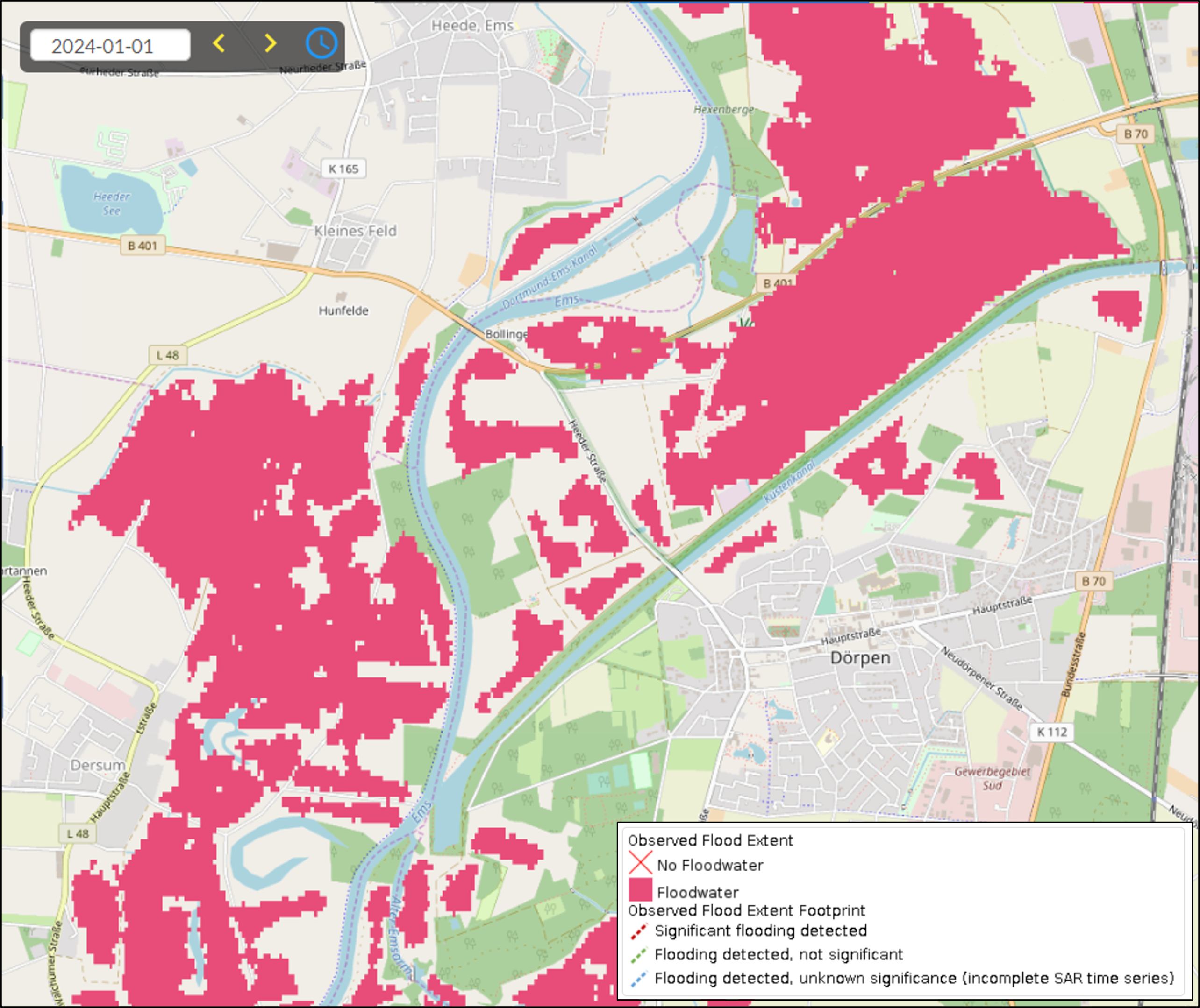
¶ 3.1. GFM output layer: Observed Flood Extent
The GFM output layer Observed Flood Extent identifies the pixels covered by floodwater, mapped using Sentinel-1 SAR backscatter intensity. An example of this output layer is shown in Figure 1. Pixels that are normally under water (identified using the monthly Reference Water Mask) are not part of this output layer. Observed Flood Extent is derived using the GFM ensemble flood mapping algorithm, as described in Section 2. To map flood extent pixels for a certain date, the algorithm uses as input the Sentinel-1 data overpass plus offline-generated Sentinel-1 SAR parameters and auxiliary thematic datasets such as Exclusion Mask and topography (e.g., DEMs and HAND index). The relative orbit path information, to select the corresponding offline-generated Sentinel-1 SAR parameters, is extracted from the Sentinel-1 Metadata. During the near real-time operation of the GFM product, the acquisition month of the Sentinel-1 scene is retrieved from the Sentinel-1 Metadata and the corresponding monthly Reference Water Mask is cropped to the extent of the processed Sentinel-1 scene. All the processing is done at the 20 metres spatial resolution of the Sentinel-1 pre-processed data cube. Flooded pixels values in the Observed Flood Extent output layer are then adjusted based on values of the Exclusion Mask and Reference Water Mask, as follows:
| Flooded pixel value: | Exclusion mask or Reference Water Mask values: | Adjusted flooded pixel value: |
| 1 (i.e. Flood) | 1 (i.e. TRUE) | 0 (i.e. No flood) |
¶ 3.1.1 Maximum Flood Extent
This second-level output layer allows users to download, for any area of interest (AOI), an automatically-generated composite showing the maximum flood extent of the available GFM output layers Observed Flood Extent, within a specific time-frame (the limit is two months). Note that the query can be submitted via both the GFM Web Portal and the REST-APIs, giving the users the options to retrieve data as vector (geojson), raster (OCG), or both formats. Further guidance on the proper use of this function is available in the GFM Quick Start Guide.
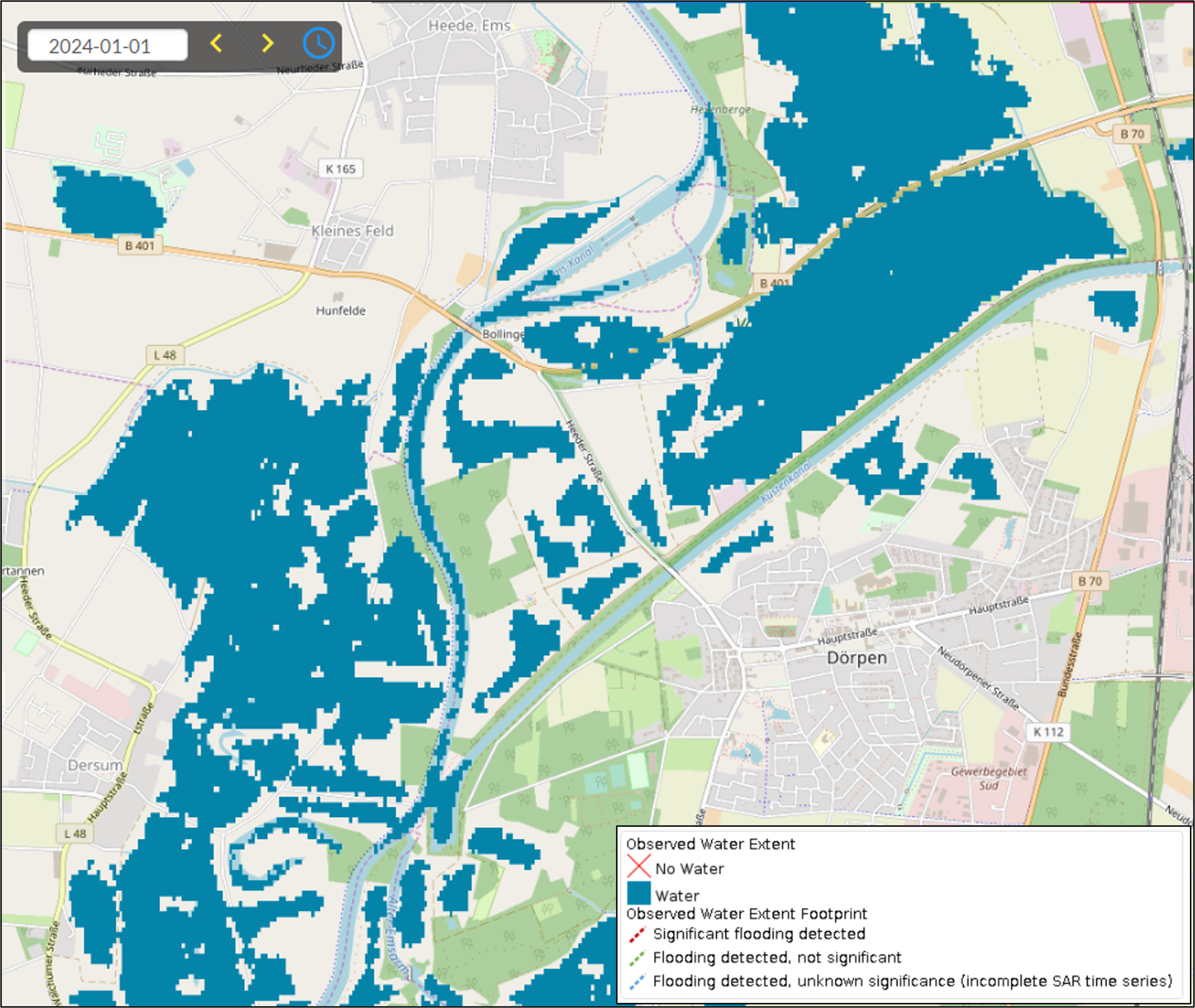
¶ 3.2 GFM output layer: Observed Water Extent
TThe GFM output layer Observed Water Extent identifies the pixels classified as open and calm water using Sentinel-1 SAR backscatter intensity and is derived using the GFM ensemble flood and water mapping algorithms. An example of this output layer is shown in Figure 2.
To map water extent pixels for a certain date, the algorithm uses as input the Sentinel-1 data overpass plus offline-generated Sentinel-1 SAR parameters and auxiliary thematic datasets such as Exclusion Mask and topography (e.g. DEM and HAND index). The relative orbit path information, to select the corresponding offline-generated Sentinel-1 SAR parameters, is extracted from the GFM output layer Sentinel-1 Footprint and Metadata. All the processing is done at the 20 metres spatial resolution of the Sentinel-1 pre-processed data cube. The GFM output layer Observed Water Extent is created as a union of the GFM output layers Observed Flood Extent (from the GFM ensemble flood mapping algorithm) and Reference Water Mask (from the GFM ensemble flood mapping algorithm), which represents the extent of open water bodies under normal conditions. In practice, reference masks of permanent water extent are often used for this purpose (Wieland and Martinis, 2019).
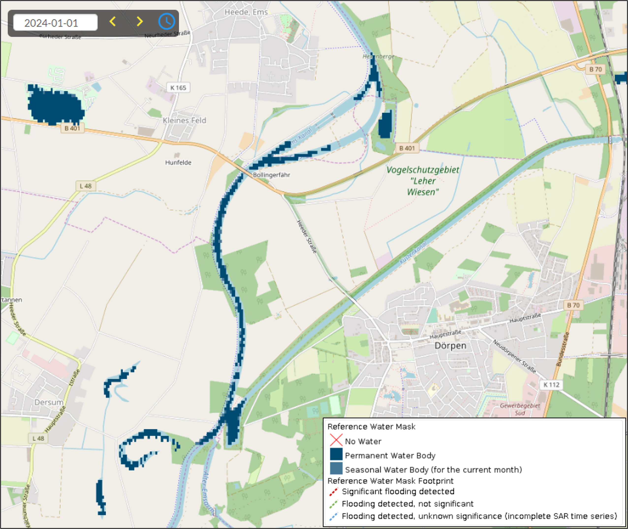
¶ 3.3 GFM output layer: Reference Water Mask
The GFM Reference Water Mask shows open and calm water (permanent and seasonal), mapped by applying the GFM ensemble water mapping algorithm to a five-year “data cube” (or time-series) of Sentinel-1 SAR backscatter intensity. An example is shown in Figure 3.
Whereas the mapping of permanent water uses as input the median backscatter of all Sentinel-1 data from a five-year period (2018-2022), the mapping of seasonal water uses the median backscatter of all Sentinel-1 data from a given month over the same five-year period. As a result, 12 masks are available, one per month, which includes information on the permanent and seasonal water extent. This parameter database is updated once a year. For example, the NRT system running in 2022 relied on the Reference Water Mask extracted from the Sentinel-1 pre-processed data cube from 2020 and 2021. Radar shadow and low sensitivity exclusion layers, and the HAND index, are applied to the reference water mask (and associated uncertainty layer) to correct pixels that were possibly misclassified. Finally, the Copernicus Global Surface Water Maximum Water Extent layer (Pekel et al., 2016) is used to remove possible false positive classifications, while the Copernicus Water Body Mask is used to correct false negatives (e.g. large lakes with roughened surface falsely classified as land) and to enforce a consistent land-sea border. A truly permanent water area would mean that there was observed water coverage in every single observation of the considered time-period, i.e., the Water Occurrence (WO), which is the ratio between the number of water detections during a certain time-period and the number of valid observations of the same period, would be 100%. To consider uncertainties in the single water segmentations and the occurrence of hydrological extreme events the WO threshold is usually relaxed to a value of 85-90 % (e.g. Pekel et al., 2016).
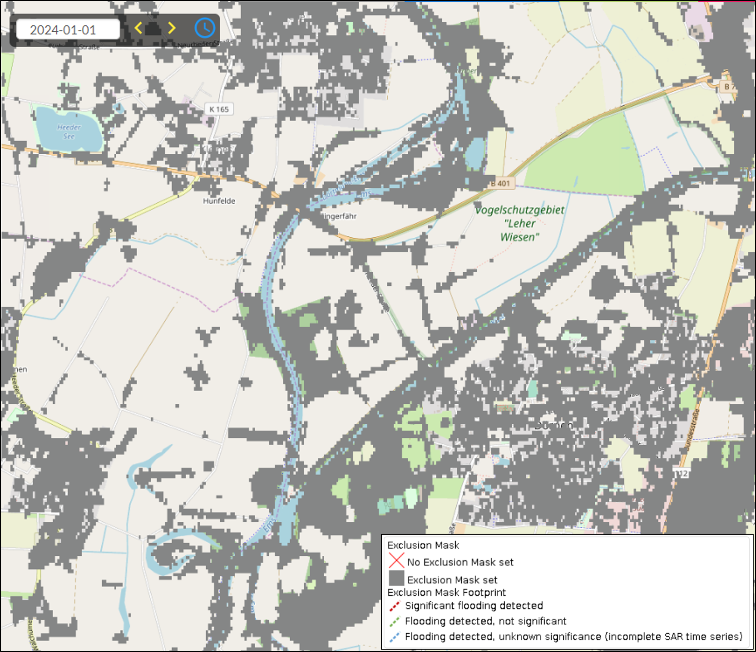
¶ 3.4 GFM output layer: Exclusion Mask
The GFM output layer Exclusion Mask indicates those locations (pixels) where the SAR data does not contain the necessary information for a robust flood delineation, due to the combined deleterious effects of the following main “static” factors:
▪ No sensitivity to flood mapping, where Sentinel-1 does not receive sufficiently strong signals from the ground surface to distinguish a flooded from a non-flooded surface.
▪ Water look-alikes, where Sentinel-1 SAR backscatter from the non-flooded ground surface is so low as to be indistinguishable from the backscatter from smooth open water.
▪ Strong topography, when Sentinel-1 signals are heavily distorted by terrain effects, effectively enhancing the noise and signal disturbances to such a degree to that it becomes larger than the change in backscatter due to potential flooding.
▪ Radar shadows, when Sentinel-1 receives no signals from certain regions of the land surface because of mountains, high vegetation canopies or anthropogenic structures.
For generation of the Exclusion Mask, the GFM product implements various methods that address the identified problems of SAR-based flood mapping. The parameter database stores for all locations, on a pixel basis, the areas excluded by the four groups of factors, with the radar shadow layer per local Sentinel-1 orbit configurations (up to six per location). During NRT operation, the relative orbit is determined from the S-1 metadata, and the respective Exclusion Mask layers are subset to the extent of the processed Sentinel-1 scene and form a single binary mask for exclusion areas. As no-sensitivity is a problem leading more often to an under-estimation rather than over-estimation of flooding (e.g. in urban areas), the no-sensitivity -masking is only applied to pixels classified as non-flooded. Pixels classified as flooded are kept unmasked. Any no-data areas from the flood mapping algorithm are forwarded to this layer and added as no-data values.
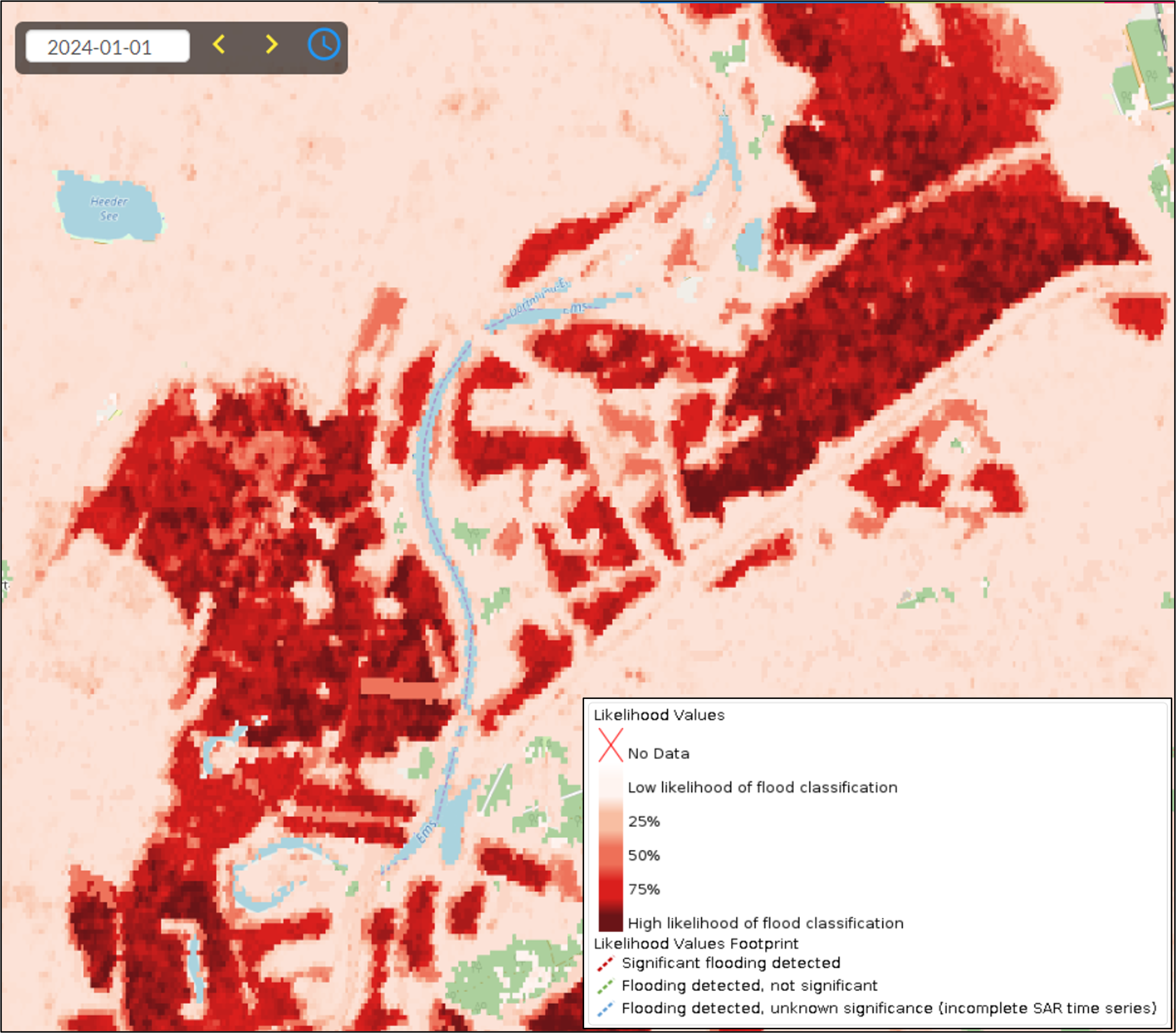
¶ 3.5 GFM output layer: Likelihood Values
Along with the binary map product (i.e. Observed Flood Extent), aggregated “likelihood” values are generated, as a simplified “appraisal of trust” in the ensemble flood mapping method. An example of this output layer is shown in Figure 5 The methods used by the three GFM flood mapping algorithms to compute the Likelihood Values for a Sentinel-1 grid-cell, and the method used by the GFM Ensemble algorithm to combine these values into a final Likelihood Value for each grid-cell, are described in the GFM Product Definition Document (PDD). Likelihood values lie in the interval 0 to 100%, where:
|
|
|
|
|
|
|
Like the GFM Observed Flood Extent output layer, the computed Likelihood Values are adjusted based on values of the Exclusion Mask, as follows.
| Flooded pixel value: | Exclusion mask value: | Adjusted flooded pixel value: | Adjusted Likelihood Value: |
| 1 (i.e. Flood) | 1 (i.e. TRUE) | 0 (i.e. No flood) | 49 (= lowest confidence for No flood) |
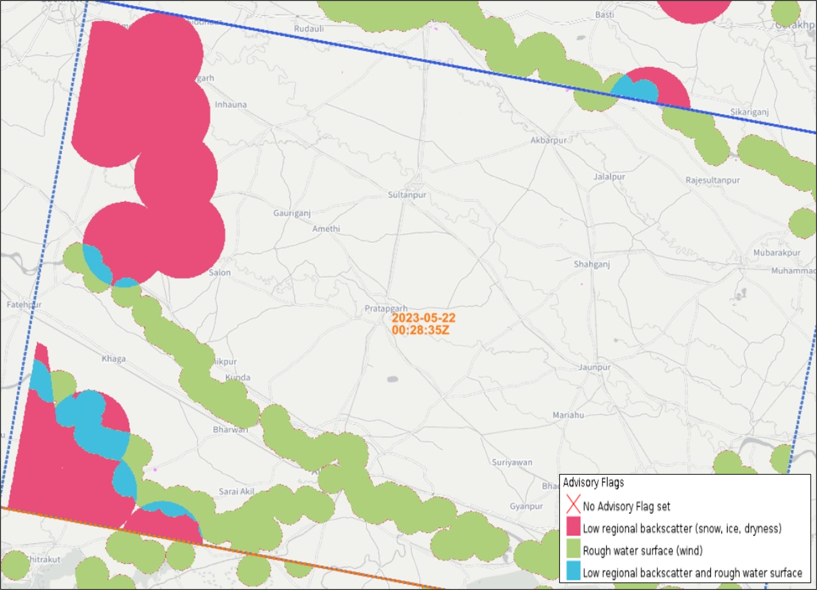
¶ 3.6 GFM output layer: Advisory Flags
The GFM output layer Advisory Flags indicates pixels that potentially suffer from decreased contrast between water and non-water surfaces due to meteorological factors as wet snow, frost and dry soil or wind-roughened water. Pixels marked by the Advisory Flags are not excluded by the Exclusion Mask, but users are advised to use with caution the GFM flood and water extent results over flagged areas. An example of this output layer is shown in Figure 6. For each incoming Sentinel-1 scene processed by the flood mapping algorithm, advisory flag information is generated in near-real time. The presence of decreased contrast between water and non-water surfaces is indicated by two distinct flags and their overlapping regions:
| The low regional backscatter flag identifies areas of low backscatter on a regional scale, which may be attributed to conditions such as dry soil, frost, or snow cover. To do this, regional backscatter for that month is compared to the incoming scene at 20 km scale. If low backscatter is detected in the incoming scene at this scale, a 14 km buffer zone is applied around the affected pixels, flagging them as areas of regional low backscatter. |
| The rough water surface flag highlights areas surrounding known water bodies that are likely affected by wind, indicating potential disturbances in the water surface. Therefore, the backscatter from known water bodies, as identified by the reference water mask, is compared to the calm water signature derived from backscatter time-series data. If a significant increase in backscatter is detected, a 5 km buffer zone around the affected water surface is flagged for potential wind impact. |
| The regions where advisory flags 1 and 2 overlap are highlighted separately. |
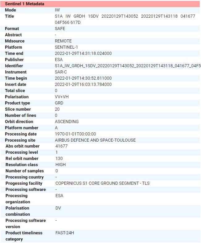
¶ 3.7 GFM output layer: Sentinel-1 Footprint and Metadata
The GFM output layer “Sentinel-1 Footprint and Metadata” shows all metadata attributes provided with each Sentinel-1 GRD data product used to generate the main GFM ain output layers. Metadata of each Sentinel-1 GRD scene are provided in the distributed Sentinel “Standard Archive Format for Europe (SAFE)” format, an XML file containing the mandatory product metadata. Examples of this output layer are shown in Figure 7 and Figure 8. The four categories of attributes in the manifest file are: (a) Summary; (b) Product; (c) Platform; (d) Instrument. Platform- and instrument-related attributes are “static” for the different Sentinel-1 satellites. There are 29 attributes in the manifest file, e.g. information on absolute orbit number, pass direction, polarisation, sensing start and end date and product timeliness category. An abstract of the included attributes is given below, as an example:
|
|
|
|
|
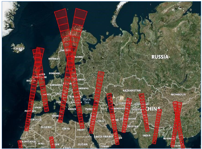
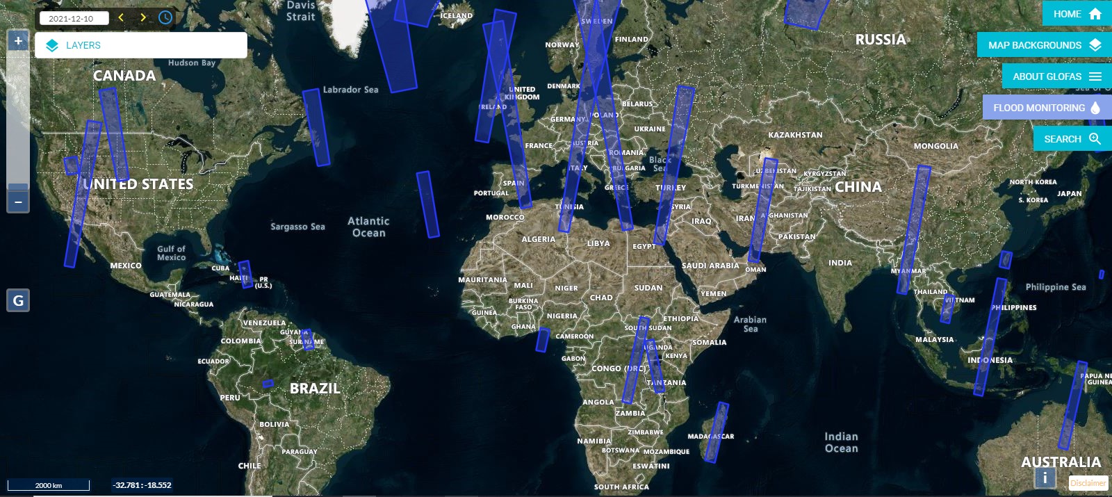
¶ 3.8 GFM output layer: Sentinel-1 schedule
Sentinel-1 observations follow a strict acquisition planning often referred to as acquisition segments. Information on the planned future acquisition is provided by ESA in form of Keyhole Markup Language (KML) files. A single file usually covers an acquisition period of about 12 days, with the start and stop time of the future planned acquisitions already given in the file name. The GFM output layer “Sentinel-1 schedule” shows planned Sentinel-1 acquisitions for the next three days. An example of this output layer is shown in Figure 9.
KML files are published regularly by ESA, well before activation, with potential last-minute changes due to requests from the Copernicus Emergency Management Service. Information provided in the KML files is organised based on the planned data takes. Parameters listed in Table 5 are included in the KML. The KML files are regularly checked and downloaded at EODC and ingested into the described metadata database for further analysis. All parameters are exposed as PostGIS layer to extract the requested schedule information indicating the next planned Sentinel-1 GRD acquisition for a given location.
|
PARAMETER |
DESCRIPTION |
|
Datatake ID: |
Unique product identifier (hexadecimal). |
|
Mode: |
Instrument acquisition mode. |
|
Observation (duration): |
Duration of the planned data take (in seconds). |
|
Observation (start): |
UTC start date and time of the planned data take. |
|
Observation (end): |
UTC end date and time of the planned data take. |
|
Orbit (absolute): |
Absolute orbit number at the start time of the data take. |
|
Orbit (relative): |
Relative orbit number at the start time of the data take. |
|
Polarisation: |
Instrument polarisation for the acquired data take. |
|
Satellite ID: |
Satellite identifier. |
|
Swath: |
Instrument swath (from 1 to 6 for SM, not applicable for IW and EW). |
Table 5: Information provided with the next planned Sentinel-1 GRD acquisition.
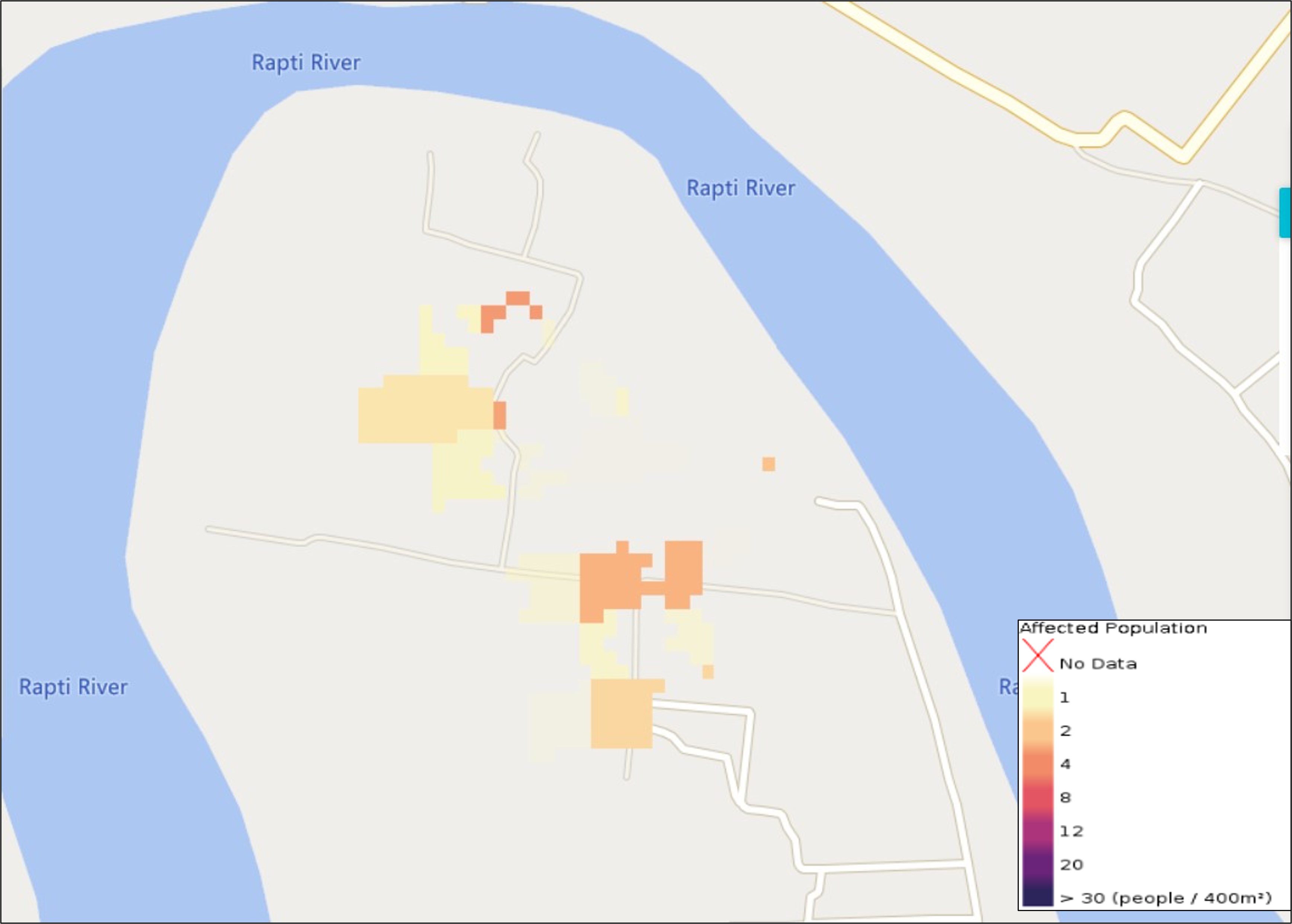
¶ 3.9 GFM output layer: Affected Population
The GFM output layer Affected Population is derived from the CEMS Global Human Settlement (GHS) layer and, in particular, from the GHS-POP dataset. This data contains a raster representation of the population's distribution and density as the number of people living within each grid cell. The information is available at various spatial resolutions and for different epochs. An example of this output layer is shown in Figure 10. For the GFM processing, the dataset at the highest possible resolution (100m) and for the latest available timestep (2020) are used. Combining this re-projected and re-sampled raster dataset and the flood extent allows to provide the number of affected people for each specific pixel detected as flooded. Note that the updated dataset replaces the former GHSL population dataset at 250m resolution with the reference year 2015, which was available at the start of GFM operations and was used for production during October 2021 – March 2023.
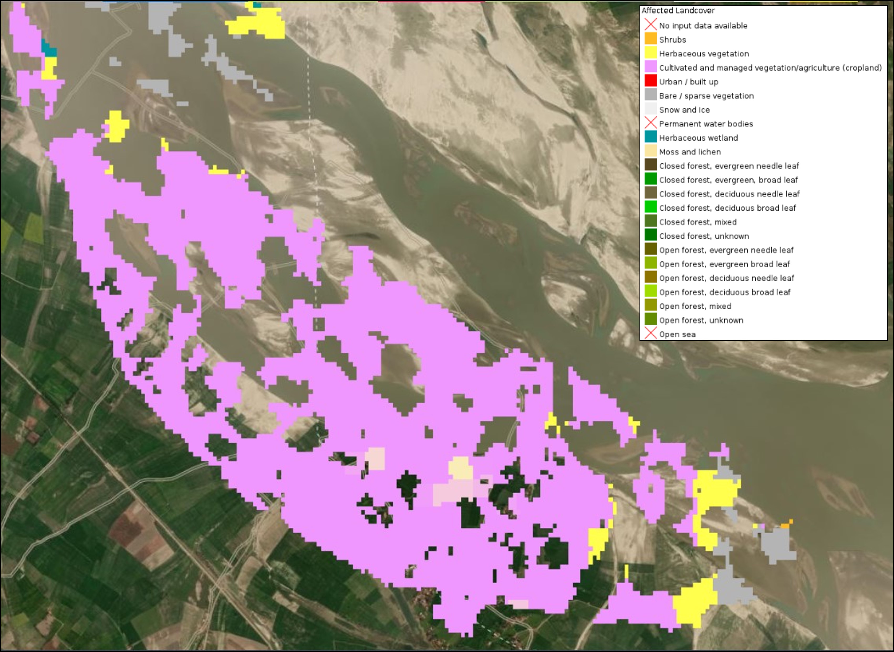
¶ 3.10 GFM output layer: Affected Landcover
The GFM product also provides, in addition to affected population, an output layer highlighting the Affected landcover for a particular flood case. This information can provide a first assessment of affected land cover or land use types, for example how much agricultural area is affected by the flood extent. An example of this output layer is shown in Figure 11. Based on the GFM consortium’s production heritage and experience in land cover mapping, this output layer is derived from the 100m-resolution database from the Copernicus Global Land Cover Service enriched with information from the Copernicus Pan-European High-Resolution Layers (i.e. Imperviousness, Forests, Grassland, Water and Wetness) over Europe. The Global Land Service includes 23 classes and provides annual updates, with an overall accuracy of 80%. The Copernicus Pan-European High-Resolution Layers have an overall accuracy of 85%+ and are available at 20 m (the 2018 version at 10 m) spatial resolution. In addition to both datasets, GFM also includes the most relevant classes from OpenStreetMap (roads, railways, etc.) to allow a first assessment of affected areas and infrastructure.
Didn't find what you were looking for? Send us a message through the contact forms:
EFAS: https://european-flood.emergency.copernicus.eu/en/form/feedback [Flood Monitoring]
GloFAS: https://global-flood.emergency.copernicus.eu/contact-us/ [Satellite-based Global Flood Monitoring]