¶ 6.6 GFM STAC Catalogue
The GFM output layers of worldwide flood-related information are also available through the GFM STAC catalogues. A STAC catalogue is a simple, flexible JSON-format file of links that provides a structure to organize and browse STAC items, where each item is a single geospatial dataset (or “spatio-temporal temporal asset”), represented as a GeoJSON feature plus date and time information, and links. Note that JSON is a text-based data format for storing and exchanging data, which is widely used for transferring data between a server and a web application. GeoJSON is an open standard, text-based format for representing simple geographical features and their non-spatial attributes, based on JSON.
In order to access and explore the GFM STAC catalogues, GFM provides a set of Jupyter notebooks (listed below), which are freely available on EODC’s GFM GitHub platform. A Jupyter notebook is a JSON-format computational notebook documents combining code (in Python), text descriptions (in Markdown), data, rich visualizations, and interactive controls. (The name Jupyter refers to the programming languages Julia, Python and R).
| download_gfm_python.ipynb |
|
| gfm_dask_objectstorage.ipynb |
|
| gfm_filter.ipynb |
|
| gfm_maximum_flood_extent_dask.ipynb |
|
| gfm_maximum_flood_extent_local.ipynb |
|
| gfm_maximum_flood_extent_simple_plot.ipynb |
|
| gfm_maximum_flood_extent_stac.ipynb |
|
| gfm_plot_flood_scene.ipynb |
|
| gfm_rfm_evaluation.ipynb |
|
¶ 6.6.1 Accessing the GFM STAC catalogues using the EODC STAC Catalogue Browser
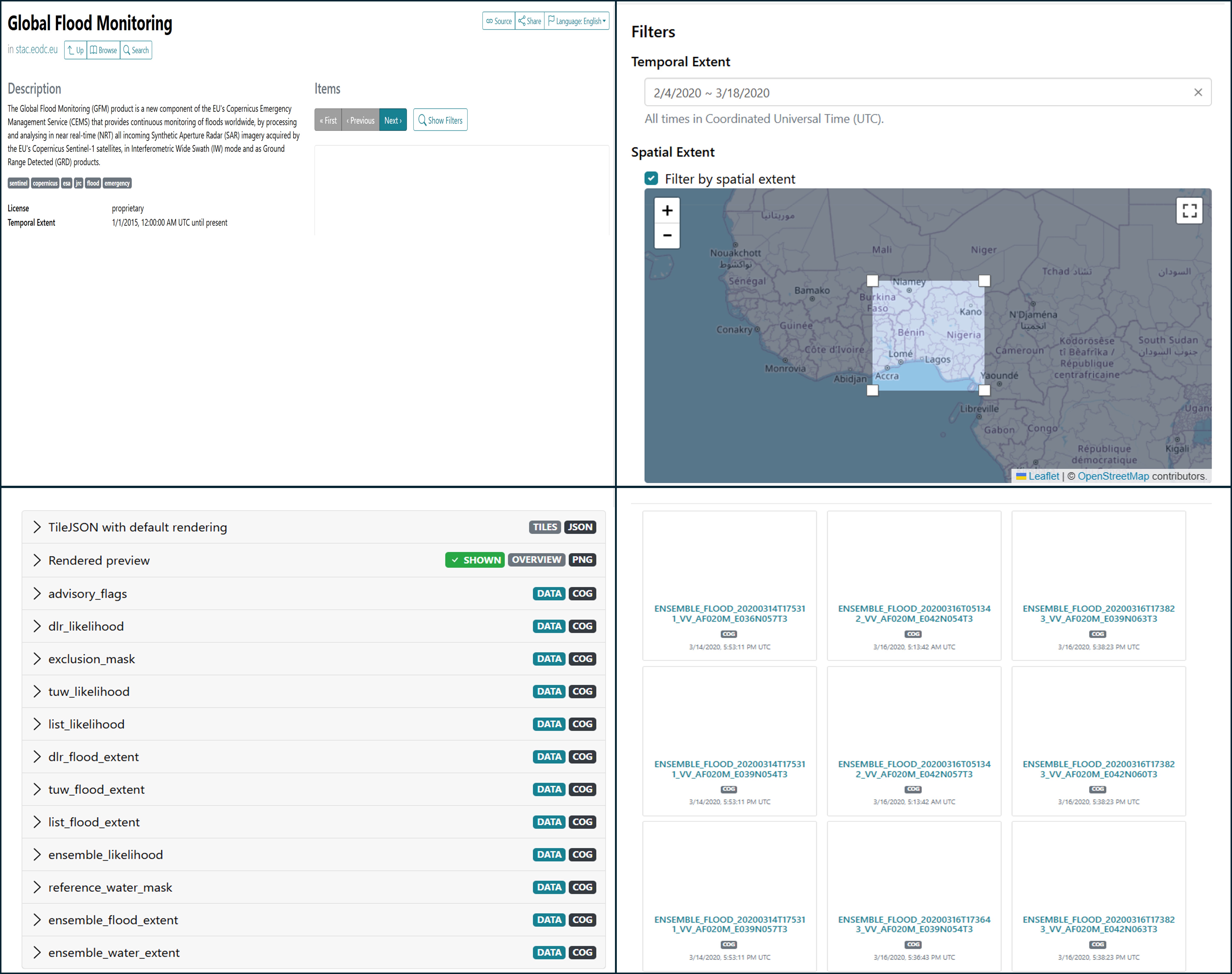
| 1. The EODC Catalogue stores all Sentinel-1 scenes. Request the latest data in the GFM STAC catalogue via the EODC STAC Catalogue browser (top left graphic below). |
| 2. By clicking on the “Search” option, specific Sentinel-1 scenes can be selected using the provided “Temporal Extent” filter to select the desired time period, and the “Spatial Extent” filter to select the desired area (top right graphic below). |
| 3. Once the desired parameters are defined, the number of results to be displayed on each page can be set (the default is 12). When the query is submitted, the retrieved results are listed (bottom left graphic below). |
| 4. By clicking on one of the retrieved scenes, all of the related assets (i.e. geospatial datasets) stored in the GFM STAC catalogue are listed (bottom right graphic below), including the intermediate products (e.g. the observed flood extent detected by each individual GFM flood mapping algorithm). |
| 5. By expanding each listed asset, the user will be presented with all the options for that specific asset (i.e. Download, Copy URL, Show on Map), and its relevant metadata. |
¶ 6.6.2 Accessing the GFM STAC catalogues using QGIS
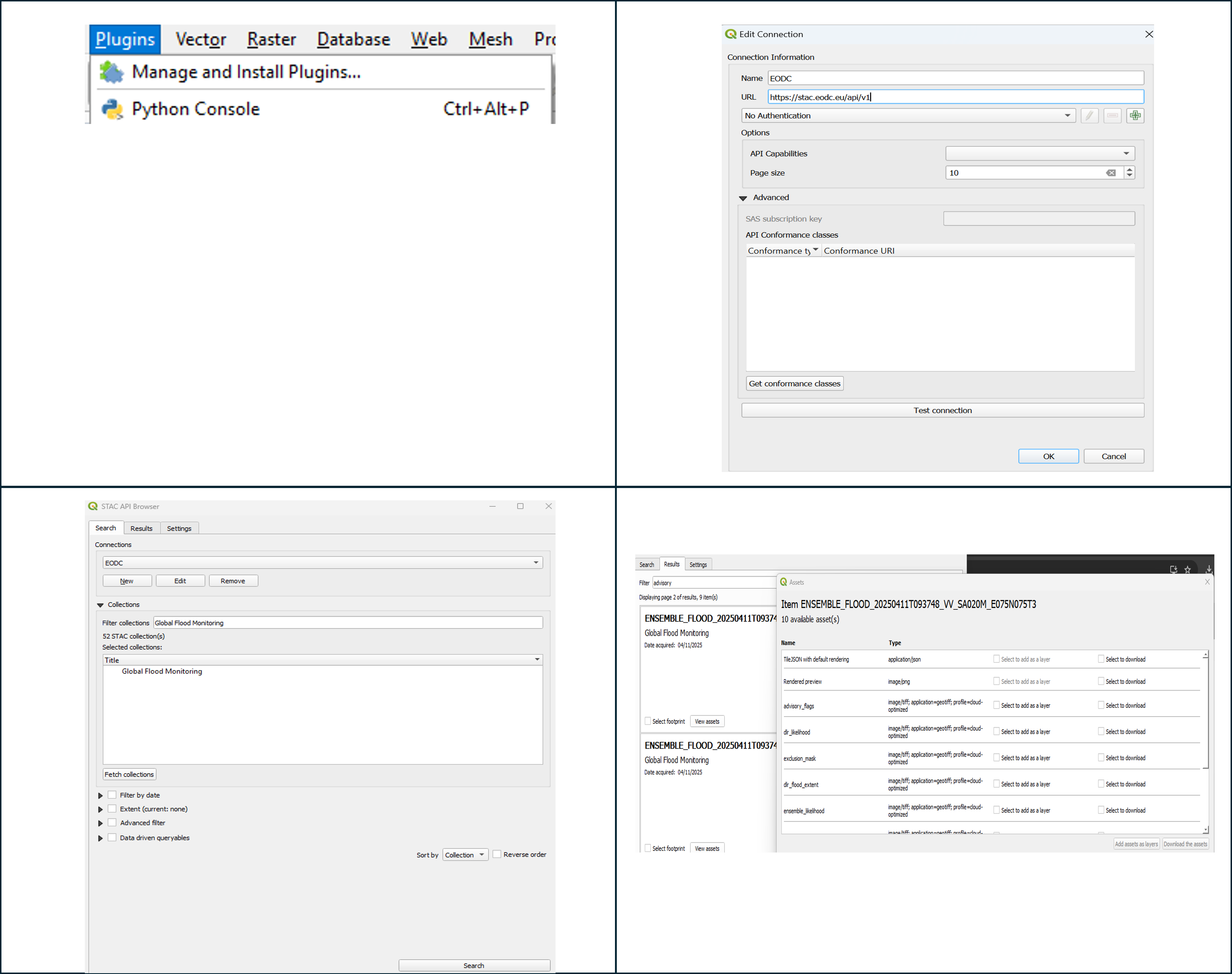
| 1. After installing QGIS, the STAC API Browser needs to be installed. In QGIS open the overview of all plugins, via “Plugins - Manage and Install Plugins” (top left graphic below). Once found, select “Install Plugin”, and close the window. |
| 2. In QGIS, create a new connection via the “New Connection” / “Edit Connection” (top right graphic below). Select a name and enter the URL. Use “Test Connection” to check that the connection works, then click on OK to create the connection. |
| 3. To display the GFM STAC catalogues, enter “Global Flood Monitoring” under “Filter Collections”, click on “Fetch collections” and “Search” (bottom left graphic below). |
| 4. The available assets corresponding with the query are listed (bottom right graphic below). Click on “View assets” to display the data or download the item. Use “Select footprint” and “Add the selected footprint” to visualise the data on the dashboard. |
¶ 6.6.3 Further sources of information on using STAC catalogues and Jupyter Notebooks
| STAC (SpatioTemporal Catalog) specification: | https://stacspec.org/en |
| Reading Data from STAC API by Microsoft Planetary Computer (with useful material to understand STAC): | https://planetarycomputer.microsoft.com/docs/quickstarts/reading-stac/ |
| Radiant Earth STAC browser, where any STAC API URL can be added (e.g. CDSE, Google Earth Engine), and the respective STAC cataloguess / items visualized: | https://radiantearth.github.io/stac-browser/ |
| EODC STAC API: | https://stac.eodc.eu/api/v1 |
| EODC’s STAC Browser: | https://services.eodc.eu/browser/#/v1/ |
| EODC knowledgebase, on how to access and work with EODC services and data: | https://docs.eodc.eu/ |
| EODC Portal (new entrypoint for EODC services), including the "Explorer", which is another way for visualizing STAC catalogues / items: | https://portal.services.eodc.eu/ |
| Jupyter Notebook documentation: |
Didn't find what you were looking for? Send us a message through the contact forms:
EFAS: https://european-flood.emergency.copernicus.eu/en/form/feedback [Flood Monitoring]
GloFAS: https://global-flood.emergency.copernicus.eu/contact-us/ [Satellite-based Global Flood Monitoring]